VDL Browser Application

1. Introduction
2. User Interface Controls
3. Selecting Units and Viewing Data
4. Labelling Data
5. Viewing Model Information
6. Filtering and Re-Filtering Data
7. The Browse Tool
8. The Partition Tool
9. The Zoom Tools
10. The Navigation Tool
11. The Sequence Model Editor Tool

1. Introduction

The Visualization Description Language (VDL) is an XML tag-based language for describing interactive visualizations. VDL visualizations or models are implementation language independent visual descriptions of data.

This document describes the VDL Browser application. The VDL Browser is a prototype VDL rendering tool that performs the following roles:

• displaying models written in the Visualization Description Language (VDL);
• providing commonly used visualization tools for examining the structure and data in VDL models, including browsing and partitioning data, and requesting details on demand; and
• providing a framework for passing data to VDL filters and displaying the results.

This document describes the facilities provided by the VDL Browser and how to use them. Section 2 describes the user interface controls. The remaining sections describe the following topics:

• selecting units and viewing data;
• data labelling;
• viewing model information;
• filtering and re-filtering data;
• browsing data with the Browse tool;
• partitioning data with the Partition tool; and
• zooming into models and navigating viewpoints with the Navigation tool.

2. User Interface Controls

2.1 The Main Window

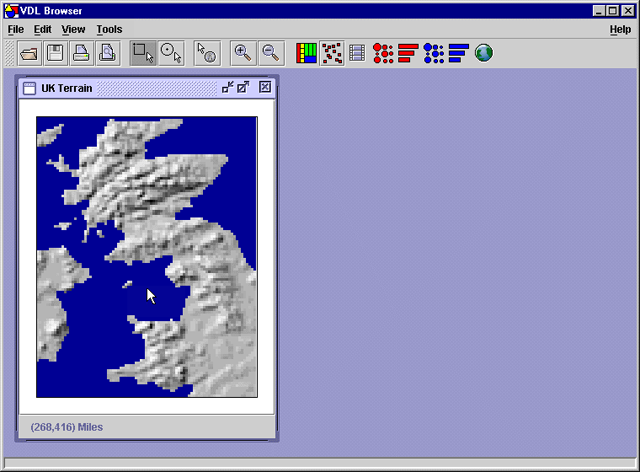
Figure 2.1 shows the VDL Browser application with a VDL model displayed in a model window. The main window has three parts:

1. menu bar;
2. tool bar; and
3. model windows.

These are described in the following sections.

Figure 2.1 – The VDL Browser application.

2.2 The Menus

The VDL Browser has the following menus:

• file menu;
• edit menu;
• view menu;
• tools menu; and
• help menu.

The File Menu

The File menu is shown in figure 2.2.

Figure 2.2 – The File menu.

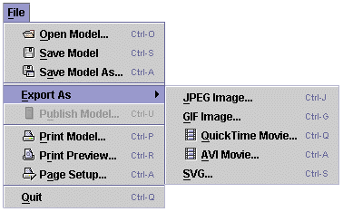
Open Model

Open a VDL Model. Models can also be opened by dragging the filename of a VDL model onto the main window of the VDL Browser.

Save Model

Save the model in the currently selected window. When a VDL model is saved, the VDL that describes the current state of the model is written to a file. All changes to the model such as changes to the model information and property values such as color changes will be saved.

Save Model As

Save the model in the currently selected window with a new file name.

Export As JPEG Image

Save a JPEG image of the model in the currently selected window.

Export As GIF Image

Save a GIF image of the model in the currently selected window.

Export As QuickTime Movie

Save the model in the currently selected window in QuickTime format. This option is only available for models with a sequence layout.

Export As AVI Movie

Save the model in the currently selected window in AVI format. This option is only available for models with a sequence layout.

Export As SVG

Save the model in the currently selected window in Scalar Vector Graphics (SVG) format.

Print Model

Print the model in the currently selected window.

Print Preview

Preview what will be printed.

Page Setup

Change the current printer settings.

Quit

Exit the VDL Browser application.

The Edit Menu

The Edit menu is shown in figure 2.3.

Figure 2.3 – The Edit menu.

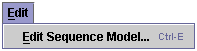
Edit Sequence Model

Display the Sequence Model Editor tool. The Sequence Model Editor tool is described in section 12.

The View Menu

The View menu is shown in figure 2.4.

Figure 2.4 – The View menu.

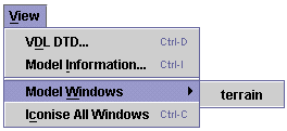
VDL DTD

Display the XML Document Type Definition (DTD) for VDL.

Model Information

Display the model information for all of the models currently opened in the VDL Browser.

Model Windows

Select a model name from this menu to bring the window containing the model to the front.

Iconize All Windows

Iconize all the model windows.

The Tools Menu

The Tools menu is shown in figure 2.5.

Figure 2.5 – The Tools menu.

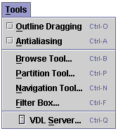
Outline Dragging

Select this checkbox to enable outline dragging of VDL model windows.

Antialiasing

Select this checkbox to render VDL models with antialiasing.

Browse Tool

Display the Browse Tool. The Browse tool is described in section 7.

Partition Tool

Display the Partition Tool. The Partition tool is described in section 8.

Navigation Tool

Display the Navigation Tool. The Navigation tool is described in section 10.

Filter Box

Display the Filter Box. The Filter Box is described in section 6.1.2.

VDL Server

Display the VDL Server window. The VDL Server is described in section 11.

The Help Menu

The Help menu is shown in figure 2.6.

Figure 2.6 – The Help menu.

About

Display information about the VDL Browser application.

Topics

Display a list of help topics available for the VDL Browser application.

2.3 The Toolbar

Figure 2.7 shows the VDL Browser toolbar. The icons on the toolbar provide four sets of operations:

• file operations
• selection operations
• zooming operations
• VDL filters

Figure 2.7 – The toolbar.

The File Operations

The file operations are also available from the File menu.

Open

Open a VDL model. Equivalent to File>Open.

Save

Save the model in the currently selected window. Equivalent to File>Save.

Print

Print the model in the currently selected window. Equivalent to File>Print.

Print Preview

Preview what will be printed. Equivalent to File>Print Preview.

The Selection Operations

The selection operations enable VDL objects to be selected and enable their data to be examined.

Select the Rectangular Selection tool.

Select the Circular Bullseye Selection tool.

Select the XML Data Brushing tool.

The Zooming Operations

The zooming operations enable the user to zoom in on VDL objects. The zoom tools are described in section 10.

Select the Zoom In tool.

Choose the Zoom Out tool.

VDL Filters

The VDL Browser has the following VDL filters that transform data into VDL models.

Space Filler Filter

Drag a directory onto this icon to create a Space Filler visualization of the files in the directory.

Scatter Plot Filter

Click this button to create a scatter plot visualization of the data on the clipboard.

Sequence Filter

Drag a directory containing VDL models onto this icon to create a new sequence model. Each model in the directory will be contained in a group with a sequence layout. Each model will become a frame in the sequence. The order of the models in the sequence is the order in which they were last modified, i.e. the oldest VDL model file will be the first in the sequence.

Cache Matrix Chart Filter

Drag a file containing cache log data onto this icon to create a Matrix Chart visualization of the data in the file.

Cache Bar Chart Filter

Drag a file containing cache log data onto this icon to create a Bar Chart visualization of the data in the file.

Document Matrix Chart Filter

Drag a file containing document data onto this icon to create a Matrix Chart visualization of the data in the file.

Document Bar Chart Filter

Drag a file containing document data onto this icon to create a Bar Chart visualization of the data in the file.

Geographical Names Information Service (GNIS) Filter

Drag a file containing GNIS data onto this icon to create a visualization of the data in the file.

2.4 The Model Windows

VDL models are displayed in two types of window:

1. regular model windows; and
2. sequence model windows.

The type of window depends on whether a VDL model contains a sequence, i.e. a group with a sequence layout.

Regular Model Windows

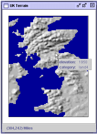
All models except sequence models are displayed in the type of window shown in figure 2.8. Figure 2.8 shows the UK Terrain model. Every VDL model is displayed with a white border around it.

Figure 2.8 – A regular model window containing the UK Terrain model.

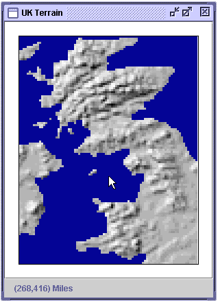
The name of the model is UK Terrain and it is displayed at the top of the window. The name of the model is specified by the name attribute of the model tag.

<model name="UK Terrain" units="Miles" scale="0.5">
   ...
</model>

As the cursor moves over the model window its current position is displayed in the bottom left of the window as (x,y) co-ordinates. The co-ordinate origin is the top-left hand corner of the model. The units of the UK Terrain model are called Miles and are specified by the units attribute. The mapping from pixels to miles is 0.5 and is specified by the scale attribute. In this model 1 pixel represents 0.5 miles.

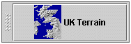
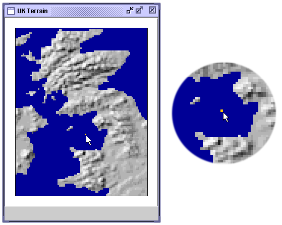
All model windows can be minimized, maximised and iconised using the controls in the top right hand corner of the window. When model windows are iconised, the icon displayed is a miniature of the model as shown in figure 2.9.

Figure 2.9 – An iconised model window showing a miniature of the model.

Sequence Model Windows

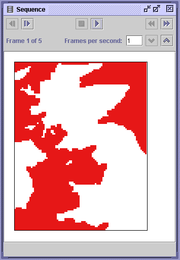
Sequence models are VDL models that contain a group with a sequence layout. Sequence models are displayed in windows with extra controls for playing the sequence. A sequence model window is shown in figure 2.10. Figure 2.10 shows the Edinburgh Sequence model created by the Sequence filter.

Figure 2.10 – A sequence model window.

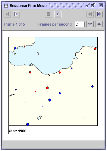
The following controls are provided for playing sequences:

Step Backward

Move to the previous frame in the sequence.

Step Forward

Move to the next frame in the sequence.

Play

Play the sequence.

Stop

Stop the sequence playing.

Rewind

Move to the first frame in the sequence.

Fast Forward

Move to the last frame in the sequence.

The rate at which frames are displayed is controlled by the value of the Frames per second input box. A new value can be typed in or the current value can be increased or decreased by one frame at a time by pressing the or buttons, respectively.

A sequence can be exported as a QuickTime or an AVI format movie by choosing File>Export As>QuickTime Movie or File>Export As>AVI Movie.

3. Selecting Units and Viewing data

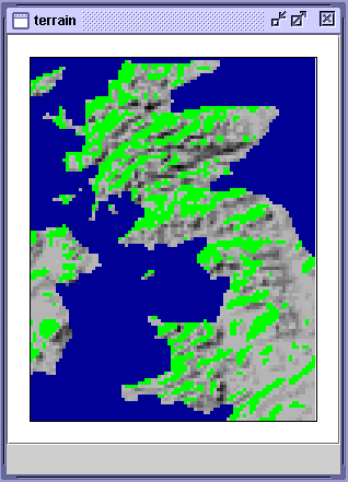
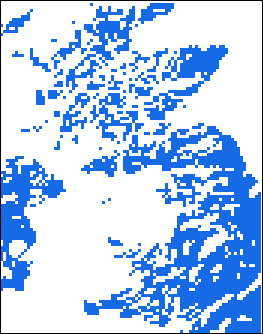
The UK Terrain Model will be used to demonstrate how units are selected and how data is viewed. The UK Terrain model is built from a large number of units with a square rectangle visual presentation. Each unit is either blue to represent the sea, or a shade of grey that is proportional to the elevation of the area it represents.

3.1 Selecting Units

The VDL Browser provides four methods for selecting units:

1. selecting individual units;
2. using the Rectangular Selection tool;
3. using the Circular Bullseye Selection tool; and
4. selecting labelled units.

Selecting Individual Units

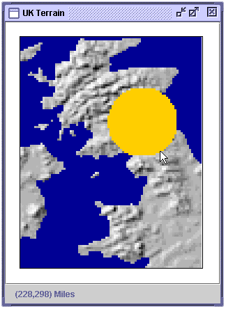
The simplest way to select a unit is to click the mouse on its visual presentation. Selected units are colored orange to indicate they are selected. Units are deselected by clicking the mouse in the white border around the model. Figure 3.1 shows a single selected unit in the UK Terrain model.

Figure 3.1 – Single unit selection.

The Rectangular Selection Tool

The Rectangular selection tool enables a rectangular region to be selected. The mouse button is clicked to fix the origin of the selection. The mouse is then dragged to increase or decrease the size of the region. Releasing the mouse selects all the units in the region enclosed by the rectangle. Figure 3.2 shows a region being selected (a) and the resulting selected units (b).

Figure 3.2 – Selection with the rectangular selection tool.

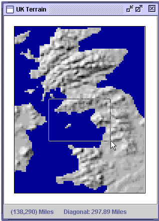
(a)

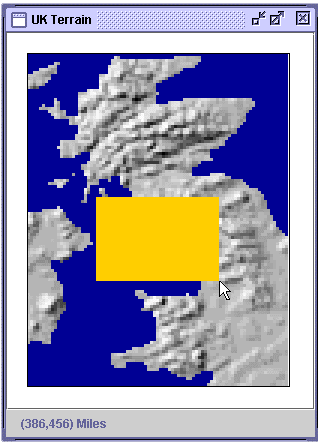
(b)

The co-ordinates of the origin of the selection and the length of the diagonal of the selection are displayed at the bottom of the window. The UK Terrain model uses miles as the units so the co-ordinates of the selection origin and the length of the diagonal are displayed in miles.

The Circular Bullseye Selection Tool

The Circular Bullseye Selection tool enables a circular region to be selected. The mouse button is clicked to fix the origin of the selection which is the centre of the circle. The mouse is then dragged to increase or decrease the radius of the selection. Releasing the mouse selects all the units in the region enclosed by the circle. Figure 3.3 shows a region being selected (a) and the resulting selected units (b).

Figure 3.3 – Selection with the circular bullseye selection tool.

(a)

(b)

The co-ordinates of the origin of the selection and the length of the radius of the selection are displayed at the bottom of the window in miles.

Selecting Labelled Units

Figure 3.4a shows the New Hampshire model partitioned by county name.

A set of labelled units can be selected in one operation by clicking the label. Figure 3.4b shows that all of the units that represent the physical and cultural features in Merrimack county have been selected by being colored orange.

Figure 3.4 – Selecting labelled units.

(a) The units of the New Hampshire model partitioned and labelled by county name

(b) Selecting the label of a partition selects all the units in the partition

3.2 Viewing Data

XML data is attached to a unit with the data tag. The UK Terrain model, for example, has two data tags that record the elevation of each tile (elevation) and one of five categories that the elevation falls into (category).

<unit name="tile">
   <presentation>
     <visual type="rectangle" width="3" height="3"
             color="180:180:180" border="false" />
   </presentation>
   <data>
      <category>land4</category>
      <elevation>1950</elevation>
   </data>
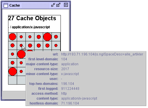
</unit>

The data of a unit is viewed using the XML data brushing tool . When the XML data brushing tool is selected, pressing and holding the right mouse button over a unit will display an XML data popup window at the bottom right of the cursor. The data tag names are displayed in bold on the left of the pop-up window. The corresponding data field values are displayed on the right. Figure 3.5a shows an example of a data window from the UK Terrain model. If a unit has no data, the popup window shown in figure 3.5b will be displayed.

Figure 3.5 – Popup XML data windows.

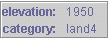
(a)

(b)

The data window will be displayed until the mouse button is released or the unit is no longer under the cursor. Dragging the mouse over another unit while the right mouse button is still pressed will display the data of the unit currently under the cursor.

The following VDL models will be used to highlight viewing data:

• UK Terrain;
• Cache Matrix Chart;
• Computer Network;
• New Hampshire; and
• UK Network.

UK Terrain Data

Figure 3.6 shows the data window for a unit in the UK Terrain model.

Figure 3.6 – The XML data window for the UK Terrain model.

Cache Matrix Chart Data

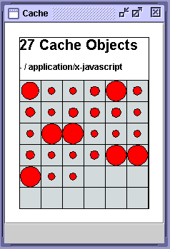
Figure 3.7a shows a small Cache Matrix Chart model. Figure 16b shows the XML data window for this model.

Figure 3.7 – The XML data window for the Cache Matrix Chart model.

(a)

(b)

Computer Network Data

Figure 3.8 shows the Computer Network model that presents four simple subnets. Each subnet contains a number of workstations connected to a server with different types of network protocols.

Figure 3.8 – The Computer Network model.

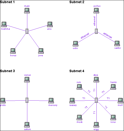
Figure 3.9a shows the XML data window of the unit that produced the title Subnet 1. Figure 3.9b shows the XML data window for the unit that produced the client machine called mars. Figure 3.9c shows the XML data window for the unit that produced the link with the label ethernet.

Figure 3.9 – The XML data windows for the Computer Network model.

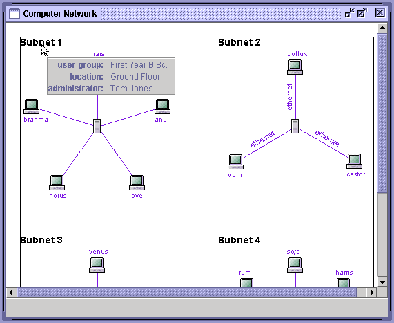
(a)

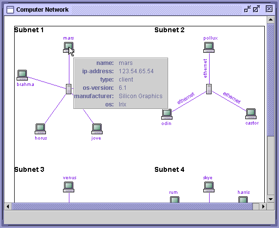
(b)

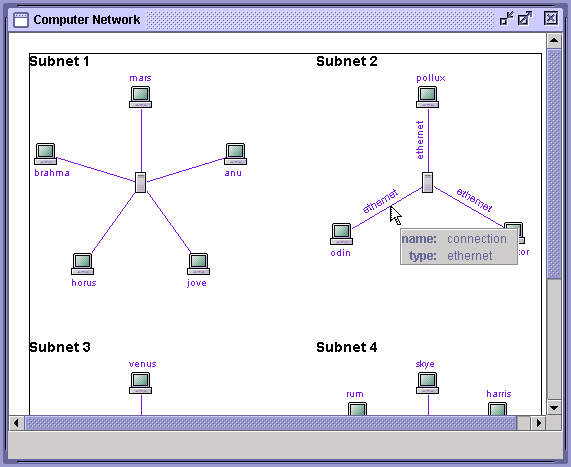
(c)

New Hampshire Data

Figure 3.10 shows the New Hampshire model. Figure 3.10a shows the XML data window for the New Hampshire model when the cultural and physical features are presented as data points. Figure 3.10b shows the XML data widow when the features are presented as icons.

Figure 3.10 – The XML data windows for the New Hampshire model.

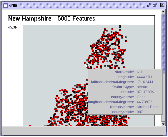
(a)

(b)

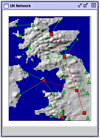
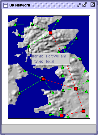
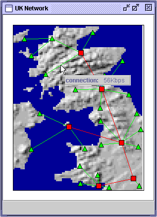
UK Network Data

Figure 3.11a shows the UK Network model. Figures 3.11b and 3.11c show the XML data windows for the UK Network model.

Figure 3.11 – The XML data windows for the UK Network model.

(a)

(b)

(c)

4. Labelling Data

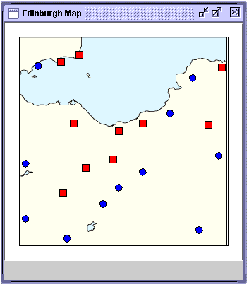
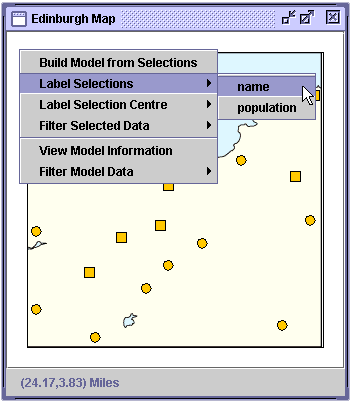
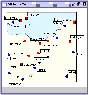
Figure 4.1a shows the Edinburgh Region model that will be used to demonstrate data labelling. The Edinburgh Region model displays several cities and towns in the Edinburgh area as squares and circles, respectively. Each city and town has data tags that records its name and population. The data for each town and city records the name and population with the name and elevation tags, respectively.

<data>
   <name>Edinburgh</name>
   <population>450000</population>
</name>

Selected data points can be labelled with the value of one data tag value at a time, in this case either the name of the city or town or its population. The data points to label are first selected using the rectangular or circular bullseye selection tools. Next, right-clicking on the border around the model will display the popup menu shown in figure 4.1b. The Label Selections option lists the XML data tag names for the data points, in this case, name and population. Selecting name will label each selected data point with the value of the name data tag, as shown in figure 4.1c. The label layout algorithm attempts to minimize the amount of overlapping.

Figure 4.1 – Labelling data.

(a)

(b)

(c)

5. Viewing Model Information

Model information is viewed with the model information dialog. The model information dialog is displayed with View>Model Information and is shown in figure 5.1.

Figure 5.1 – The model information dialog.

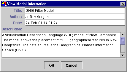
The titles of the models currently opened in the VDL Browser are displayed in the list at the top of the dialog. Selecting a title will display the details of the model in the bottom half of the dialog. The dialog displays the values of the title, author, date and description information tags of the currently selected model.

<model>
   <information>
      <title>GNIS Filter Model</title>
      <author>Jeffrey Morgan</author>
      <date>24-Feb-01 14:31:24</date>
      <description>
          A Visualization Description Language (VDL) model of New Hampshire.
          The model shows the placement of 5000 geographical features in New
          Hampshire. The data source is the Geographical Names Information
          Service (GNIS)
      </description>
   </information>
   ...
</model>

The information can be edited by changing the displayed values. The updated values will be saved when the VDL model is saved.

6. Filtering and Re-Filtering Data

This section explains how to filter and re-filter data with the VDL Browser.

6.1 Filtering Data

New VDL models can be created by passing data through a VDL filter. Users interact with two types of VDL filter:

1. copy and paste filters; and
2. drag and drop filters.

Both types of filter have an icon. Copy and paste filters are presented as push buttons with the icon as the label of the button. Figure 6.1a shows the Scatter Plot filter as an example of a copy and paste filter. The input to a copy and paste filter is the data on the clipboard. Users select appropriate data for the filter in an application and click the button with the filter’s icon.

Drag and drop filters are presented as labels onto which input data files and directories are dragged. Figure 6.1b shows the Space Filler filter as an example of a drag and drop filter. Users drag a file or directory with appropriate content for the filter onto the filter’s icon.

Figure 6.1 – VDL filter icons.

(a) The push button of a copy and paste filter.

(b) The label of a drag and drop filter.

Some VDL filters require parameter values to be set by the user to enable the filter to generate a model. If a VDL filter has parameters, a dialog will be displayed immediately after the user has either pasted data into the filter or by dragging a file or directory onto the filter.

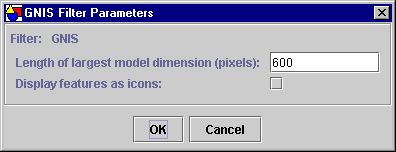
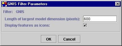
Figure 6.2 shows the parameter dialog for the Geographical Names Information Service (GNIS) filter. The GNIS filter has two parameters that control the size of the model to be created and whether the geographical features should be displayed as icons or as simple data points, respectively. This dialog captures an integer value and a Boolean value.

VDL filter parameter dialogs can capture several types of data:

• string;
• integer;
• double;
• Boolean; and
• enumerated values.

Enumerated values are a list of string values from which one must be selected.

String, integer and double parameter values are entered into an input box. Boolean parameter values are presented as a check box. Enumerated parameter values are presented as options selected with a combo box.

Figure 6.2 – The GNIS filter parameter dialog.

VDL filters are available in two parts of the VDL Browser:

1. the toolbar; and
2. the Filter Box.

All of the filters are available in both the toolbar and the Filter Box but their behaviour after creating a model is slightly different as is now described.

The Toolbar Filters

When a model is created with a VDL filter on the toolbar, the resulting VDL model is loaded directly into the browser.

The Filter Box

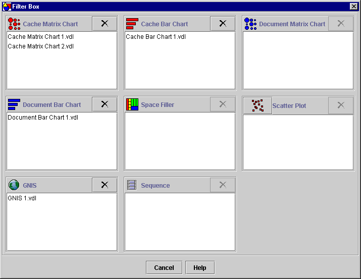
When data is pasted into or dragged onto a VDL filter on the toolbar, the resulting VDL model is loaded directly into the browser. The Filter Box enables models created with VDL filters to be stored rather than loaded directly into the browser. The Filter Box is displayed with Tools>Filter Box and is shown in figure 6.3. Each filter is displayed in a separate box. The name and icon of the filter is displayed above a scrolling list of the filenames of the VDL models created with the filter.

VDL models are created with filters in the Filter Box with the same user interaction as the filters in the toolbar, i.e. through drag and drop or copy and paste. The difference is that the models are not opened in the VDL Browser. The filename of the model is added to a scrolling list of filenames in the panel below the name and icon of the filter. The filenames can be dragged onto the main window of the VDL Browser when they are needed. This enables a set of models to be created and stored without opening them in the Browser as soon as they are created. The models listed below the name and icon of a filter can be deleted by pressing the button.

Figure 6.3 – The Filter Box.

6.2 Re-Filtering Data

Re-filtering is a generic operation that can be applied to any VDL model with data that was created by a VDL filter.

New Hampshire Geographical Features

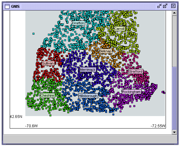
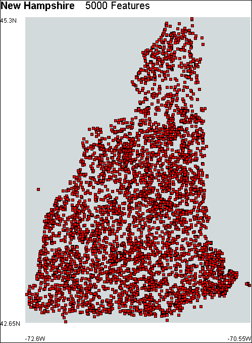
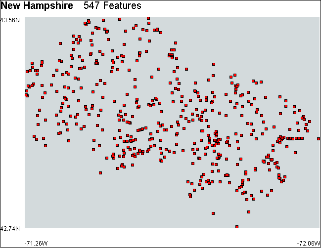
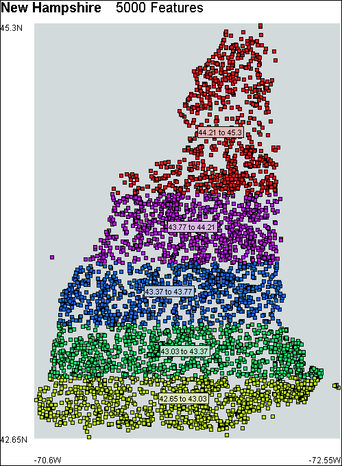
Figure 6.4 shows the New Hampshire model that will be used to demonstrate re-filtering data. The New Hampshire model was created by the Geographical Names Information Service (GNIS) filter and shows 5000 physical and cultural features of New Hampshire.

Figure 6.4 – The New Hampshire Geographical Names Information Service (GNIS) model.

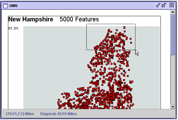
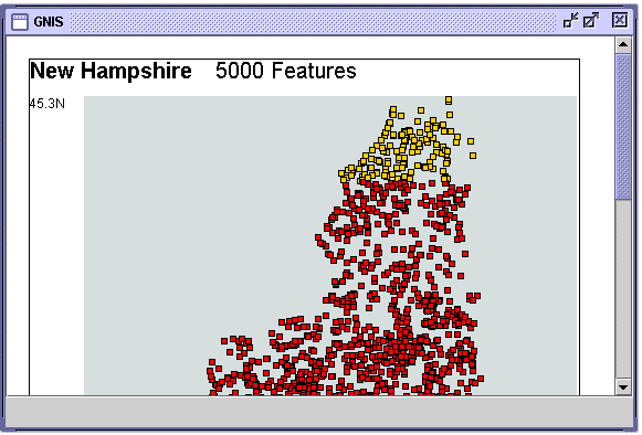
Any VDL filter can accept data selected from a VDL model that it produced. To demonstrate re-filtering, a set of selected data points in the New Hampshire model will be re-filtered with the GNIS filter. Figure 6.5 shows the selection of a set of data points in the New Hampshire model (a) and the resulting selected units (b).

Figure 6.5 – Selecting data points in the New Hampshire model.

(a)

(b)

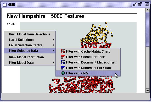
Next, right-clicking the mouse in the border around the model will display the popup menu shown in figure 6.6. The Filter Selected Data menu lists the available filters. The selected data points are passed through the GNIS filter by selecting the Filter with GNIS option. Figure 6.2 shows the GNIS filter parameters dialog box that will be displayed. After choosing a size for the model and leaving the Display features as icons option un-checked, the model shown in figure 6.7 will be produced and opened in the VDL Browser.

Figure 6.6 – Re-filtering the selected data.

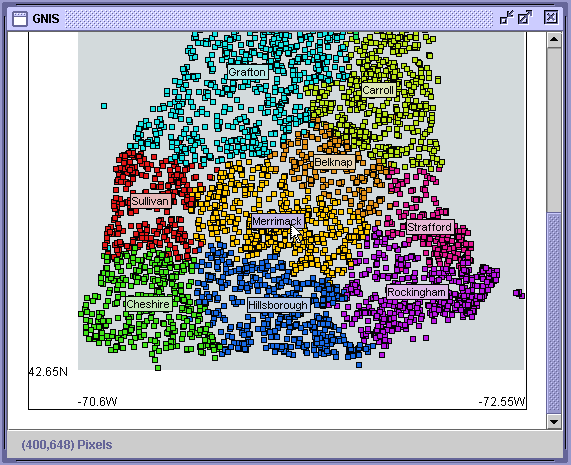
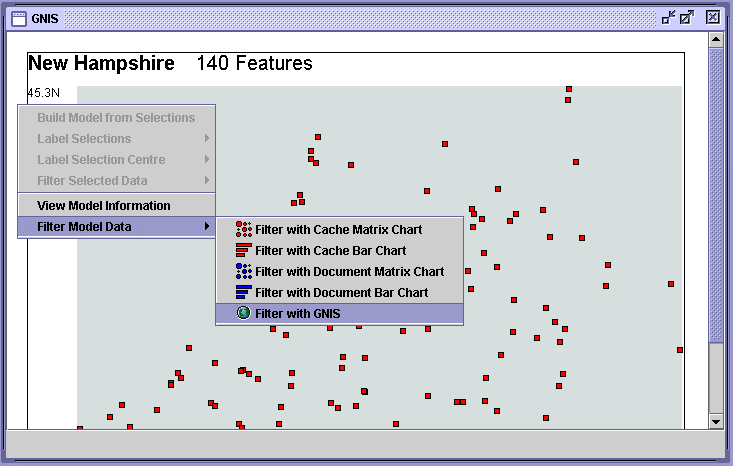
When there are a large number of features in a GNIS model, the features are best presented as data points as shown in figure 6.4. The features in the model shown figure 30 can be presented as icons by passing the all of the data in the model through the GNIS filter with the Display features as icons parameter checked. All the data in a model can be filtered without needing to select it by right-clicking the mouse in the border around the model and choosing Filter Model Data. To re-filter all the data through the GNIS filter, select Filter Model Data>Filter with GNIS as shown in figure 6.8.

Figure 6.7 – The new model produced by re-filtering the selected data.

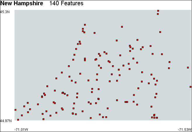
Figure 6.8 – Re-filtering the new model.

A new model with features represented by icons will be created by choosing a size for the model and checking the Display features as icons option as shown in figure 6.9.

Figure 6.9 – The GNIS filter parameters dialog.

The GNIS filter currently uses icons from the Java Look and Feel Repository to represent the physical and cultural features. These are placeholders that will be replaced when a suitable set of geographic icons are found. However, figure 6.10 shows that even using the GUI application icons, patterns in the data are highlighted, such as the stream feature which is represented by the information icon .

Passing a subset of the original data through the GNIS filter and maintaining or increasing the size of the model has the effect of zooming in on the data. Figure 6.10 shows that the features are spread out more than in the original model shown in figure 6.4.

Figure 6.10 – The New Hampshire model with icons representing the physical and geographical features.

Figure 6.11 shows the New Hampshire GNIS model partitioned by county name with labelled partitions. Each colored region shows the physical and cultural features in a county. A labelled set of units can be selected by clicking on the label. The selected data points can be passed through the GNIS filter by right-clicking the mouse in the border around the model and choosing Filter Selected Data>Filter with GNIS, as shown in figure 6.12. The GNIS filter parameter dialog will be displayed and a new enlarged model of the features in Merrimack county can be built by using the parameter values shown in figure 6.2. Figure 6.13 shows the resulting enlarged model of the features in Merrimack county. The features in this model can be interrogated and re-filtered as described above.

Figure 6.11 – The New Hampshire model partitioned by county name with labelled partitions.

Figure 6.12 – Re-filtering a set of selected data points with the GNIS filter.

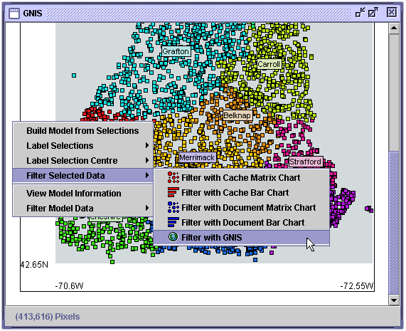
Figure 6.13 – The new model produced by filtering the selected data points with the GNIS filter.

Cache Matrix Chart Data

Figure 6.14a shows part of the Cache Matrix Chart model produced by the Cache Matrix Chart filter. Matrix charts can be very large and it is often useful to reduce the amount of data in a model by selecting some interesting data and creating a new model of that data. First select the data to be filtered, in this case the data for the unknown user (-) and the content-type application/x-javascript (shown in figure 6.14b).

Figure 6.14 – Selecting data in the Cache Matrix Chart model.

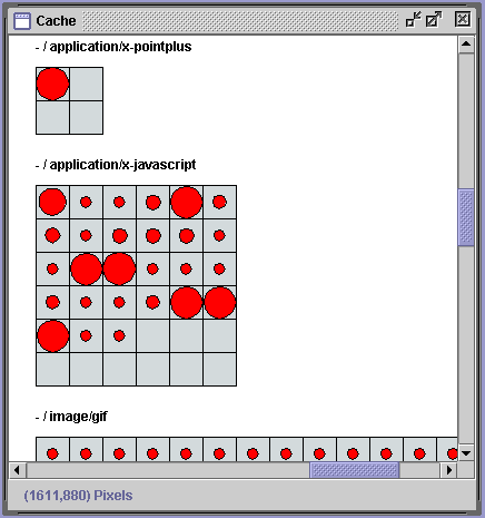
(a)

(b)

A new model of the selected data can be created by right-clicking the mouse in the border around the model and choosing Filter Selected Data>Filter with Cache Matrix Chart. The Cache Matrix Chart filter parameters dialog box shown in figure 6.15a will then be displayed. Accepting these settings produces a new model of the selected data that is shown in figure 6.16.

Figure 6.15 – Cache Matrix Chart filter parameters.

(a)

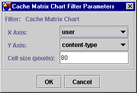
(b)

The minimum diameter of a circle in a matrix chart produced by the Cache Matrix Chart filter is 20 pixels. As the difference between values decreases, the differences between them become harder to see. Any value that maps onto a circle with a diameter of less than 20 pixels will be represented by a circle with a diameter of 20 pixels. Values that map onto circles with a diameter of 20 pixels or less cannot be differentiated.

The differences between smaller values can be differentiated by increasing the diameter of the circles in a matrix chart. The matrix chart shown in figure 16a can be enlarged by re-filtering the data in the model and increasing the value of the Cell size parameter. A new model is created by right-clicking the mouse in the border around the model and choosing Filter Model Data>Filter with Cache Matrix Chart. Using a Cell size parameter value of 80 pixels as shown in figure 6.15b will produce an enlarged model. The maximum diameter of each circle is now 80 pixels and the differences between the smaller values can be seen more easily in the enlarged model shown in figure 6.16.

Figure 6.16 – Re-filtering matrix-chart data to increase the circle diameter highlights the differences between small values.

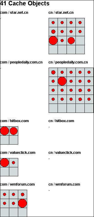
So far, only the Cell size parameter has been changed. By changing the data fields represented on the x and y axes, the data in a matrix chart can be split further. Figure 6.17 shows another part of the Cache Matrix Chart model. Here the data for user bojian and the content-type text/html. This data can be examined further by changing the data fields represented on the x and y axes, such as showing the first-level-domain on the x axis and the hostless-domain on the y axis, as shown in figure 6.18. These parameter values will produce the model shown in figure 6.19. Here we have a new view of the same data produced by re-filtering the data and changing two parameters.

Figure 6.17 – Another part of the Cache Matrix Chart model.

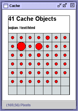
Figure 6.18 – The Cache Matrix Chart parameters dialog.

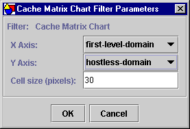
Figure 6.19 – Re-filtering to representing first-level-domain on the x axis and hostless domain on the y axis produces a new view of the data.

Cache Bar Chart Data

Any VDL filter can re-filter data selected from any model as long as the filter and the model use the same data tags. The Cache Bar Chart filter processes the same cache data as the Cache Matrix Chart filter. Therefore, any data selected in a Cache Matrix Chart model can be re-filtered with the Cache Bar Chart filter.

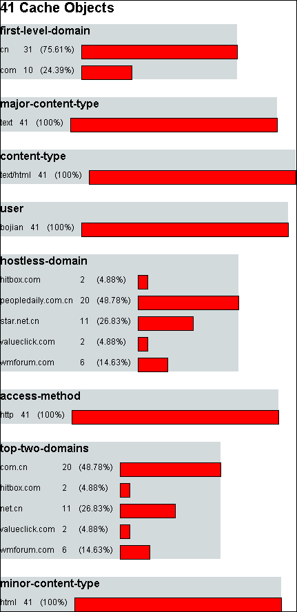
Figure 6.20 shows the data for the user bojian and the content-type text/html after it has been filtered with the Cache Bar Chart filter. The model shown in figure 6.20 was constructed by right-clicking the mouse in the border around the model and selecting Filter Model Data>Filter with Cache Bar Chart, rather than Filter Model Data>Filter with Cache Matrix Chart as has been done in the examples above.

Figure 6.20 – Cache Matrix Chart data re-filtered with the Cache Bar Chart filter.

7. The Browse Tool

The Browse tool enables a set of values to be examined, selected or filtered out. The following values can be browsed:

• the names of VDL structure elements, i.e. unit and group names; and
• XML data values contained in the data tags of a unit.

The Browse tool is displayed with Tools>Browse Tool. Figure 7.1 shows the Browse tool dialog presenting the data of the UK Terrain model.

Figure 7.1 – The Browse tool dialog presenting the data of the UK Terrain model.

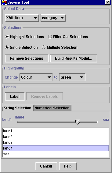
The Browse tool dialog has five areas:

1. select data area;
2. selections area;
3. highlighting area;
4. labels area; and
5. sliders and lists area.

7.1 The Select Data Area

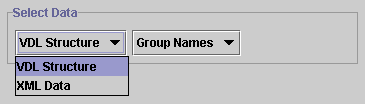
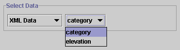
Figure 7.2a shows the select data area. The values of the combo boxes determine what aspect of the VDL model will be browsed. The selection in the left-hand combo box determines whether the VDL Structure elements or the XML Data will be browsed (figure 7.2b). If the model has no data, the XML Data option will not be available.

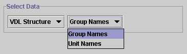
When VDL Structure is selected, the selection in the right-hand combo-box determines whether unit or group names will be browsed, as shown in the figure 7.2c. When XML Data is selected in the left hand combo box, the selection in the right-hand combo determines which of the data tags will be browsed. The UK Terrain Model has two data tags, category and elevation, as shown in figure 7.2d.

Figure 7.2 – The select data area of the Browse tool dialog.

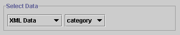
(a)

(b)

(c)

(d)

7.2 The Selections Area

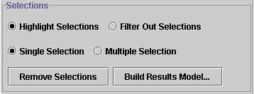
The selections area shown in figure 7.3a controls the values of two selection parameters. The first parameter determines whether selected units are highlighted by changing the color, or by filtering them out, i.e. by making them invisible. The highlighting color is controlled in the highlighting area described below.

The second parameter controls whether a single selection or multiple selections are made. When a single selection is made, any existing selection will be de-selected, and the new selection will be displayed. Multiple selection means that many selections can be shown at the same time. When a multiple selection is made, any new selections will be added to the existing selections.

Once units have been either highlighted or filtered out, the Remove Selections button enables the highlighting or filtering out to be removed to restore the model to its original state.

Figure 7.3 – The parts of the Browse tool dialog.

(a) The selections area.

(b) The highlighting area.

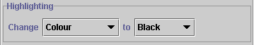
7.3 The Highlighting Area

The highlighting area shown in figure 7.3b enables you to choose how units selected with the Browse tool will be highlighted. Currently, only the color property of the unit’s visual presentation can be changed. The right-hand combo box enables you to select the color that selected units will be highlighted with.

7.4 The Labels Area

Units highlighted by browsing can be labelled by pressing the Label button. The highlighted units are taken to be a cluster and the label is centred on the centroid of the cluster.

7.5 The Sliders and Lists

The Browse tool has two sets of sliders and lists that can be used to select values: String Selection and Numerical Selection. If VDL Structure is selected in the left-hand combo box, the sliders and lists will display the names of either the units or groups, depending on the selection made in the right-hand combo box. Similarly, if XML Data is selected in the left-hand combo box, they display the values of the XML data tag selected by the right-hand combo box.

The sliders and lists display the values selected by the select data area. The sliders enable values to be selected in quick succession. As the slider is moved, the selected units will be highlighted immediately. The lists display all of the values and only one can be selected at a time.

The String Selection slider and list, shown in figure 7.3c, displays the values of the category data tag. The Numeric Selection slider and list, shown in figure 7.3d, displays the numeric values of the elevation data tag. Three matching operators are available and are selected with the combo box to the left of the slider. Numbers are matched if they are less than, equal to or greater than the selected value, as determined by the matching operator. The Numeric Selection slider and list are only available if one or more of the values contain strings that can be parsed into numbers.

7.6 Browsing the UK Terrain Model

The values of the category data tag of the UK Terrain model will be used to illustrate browsing. First 7.4a shows the Browse tool settings that will enable the category XML data tag to be browsed.

Figure 7.4 – Browsing the UK Terrain model with single selection highlighting.

(a)

(b)

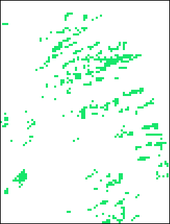
As soon as the slider is moved to the value land4, all the units with a category data tag value of land4 will be highlighted by being colored green, the color selected in the highlighting area as shown in figure 7.4b.

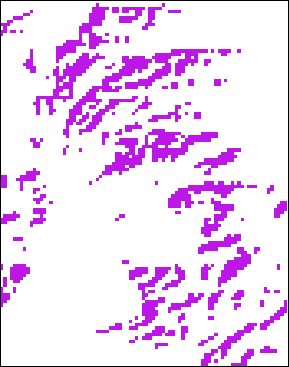
When single selection is selected, moving the slider will highlight only one value of the category tag at a time. When multiple selection is selected, all new selections will be added to the existing selections when the slider is moved. Figure 7.5a shows the Browse tool settings that will enable the UK Terrain model to be browsed with multiple selections. The highlighting color has been changed to magenta in figure 7.5a. When the category data tag value land2 is selected both land4 (green) and land2 (magenta) units are highlighted as shown in figure 7.5b.

Figure 7.5 – Browsing the UK Terrain model with multiple selection highlighting.

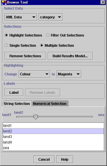
(a) The Browse tool settings for multiple selection highlighting.

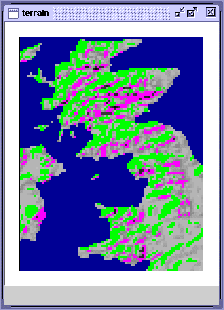
(b) The UK Terrain model with multiple selection highlighting.

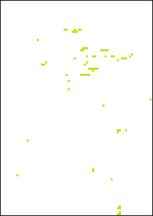
7.7 Filtering the Space Filler Filter Model

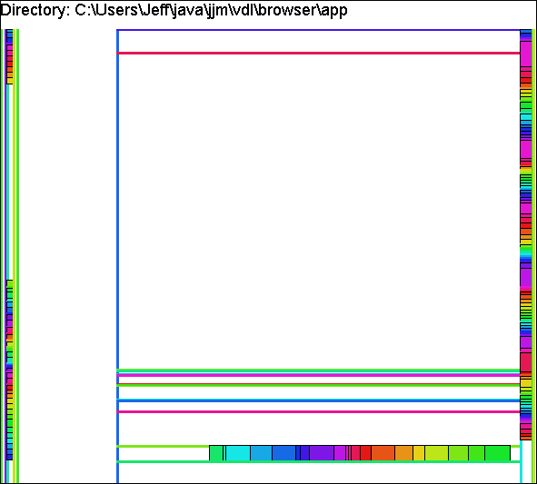
Units selected by the Browse tool can also be filtered out, i.e. made invisible. Figure 7.6a shows a Space Filler model which will be used to demonstrate filtering out. The Space Filler model was produced by the Space Filler filter.

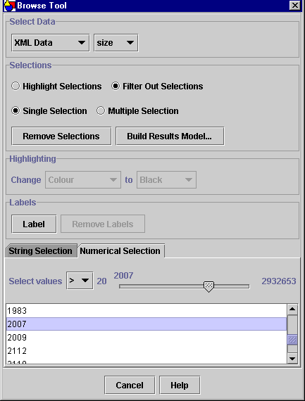
Figure 7.7 shows the Browse tool settings for filtering out all the units with a category data tag value of 2007 or greater. Figure 7.6b shows that all the units with a category data tag value of 2007 or greater have been filtered out, i.e. made invisible. Figures 7.6c and 7.6d show that all the units with a category data field value of 20000 or greater and 200000 or greater, respectively, have been filtered out.

Figure 7.6 – Filtering the Space Filler model.

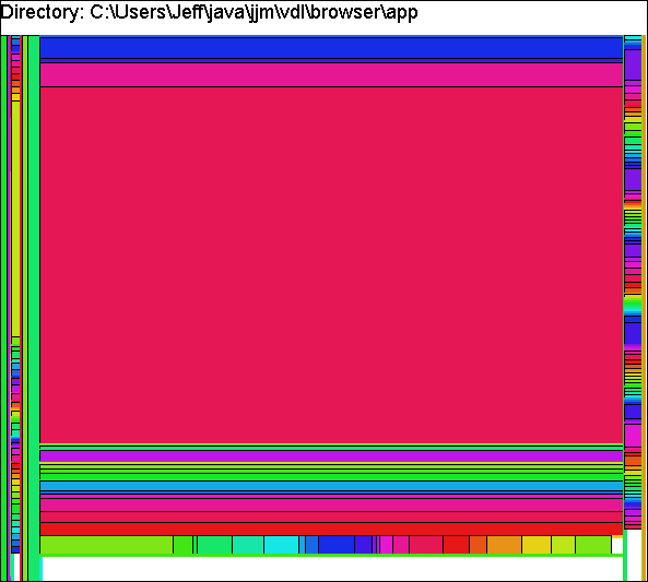
(a) The Space Filler model

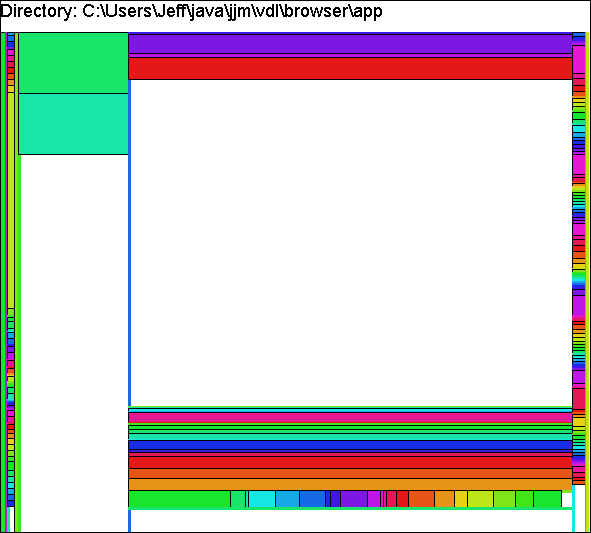
(b) The Space Filler model after filtering out units with a category data field value of 200000 or greater

(c) The Space Filler model after filtering out units with a category data field value of 20000 or greater

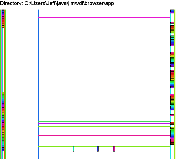
(d) The Space Filler model after filtering out units with a category data tag value of 2000 or greater

Figure 7.7 – The Browse tool dialog settings for filtering out objects in the Space Filler model with a size data tag value of 2007 or more.

8. The Partition Tool

The Partition Tool enables a set of values to be divided automatically into partitions and colored. The following values can be partitioned:

• the names of VDL structure elements, i.e. unit and group names; and
• XML data values contained in the data tags of a unit.

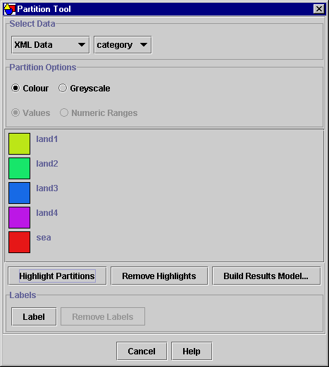
The Partition tool is displayed with Tools>Partition Tool. Figure 8.1 shows the Browse tool dialog presenting the data of the UK Terrain model.

Figure 8.1 – The Partition tool dialog presenting the data of the UK Terrain model.

The Partition tool dialog has four areas:

1. select data area;
2. partition options;
3. partition panel; and
4. labels area.

8.1 The Select Data Area

The select data area of the Partition tool is identical to the select data area of the Browse tool.

8.2 The Partition Options

Figure 8.2a shows the partition options area. The Color and Greyscale options control whether the partitioned objects are assigned a color or a greyscale value. The color and greyscale partition key panels are shown in figure 8.2b.

The Values and Numeric Ranges options control whether the objects are assigned to partitions that represent a single value or a range of numeric values. The numeric range partitioning key panel is shown in figure 8.2c.

Figure 8.2 – The parts of the Partition tool dialog.

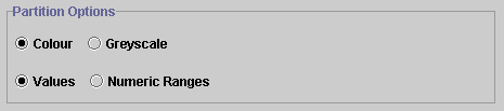
(a) The partition options.

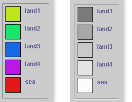
(b) Value partitioning key panel.

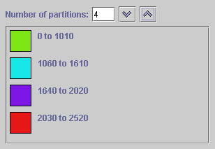
(c) Numeric range partitioning key panel.

When VDL structure or XML data—as controlled by the select data area—is partitioned as Values, literal string matching is performed. When the selected VDL structure or XML data values are partitioned as Numeric Ranges, the Partition tool will examine the values and determine if the set contains any numbers. If the set contains strings that can be parsed into numbers, the Numeric Ranges option will be made available and any numbers will be able to be partitioned numerically.

The number of numeric partitions is controlled by the value of the Number of partitions input box. A new value can be typed in or the current value can be increased or decreased by one partition at a time by pressing the and buttons, respectively.

8.3 The Partition Panel

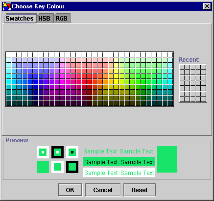
The key panel displays a square filled with the color or the greyscale value of each partition next to the value that the partition represents. The colors and the greyscale values are assigned automatically. The color or greyscale value of a partition can be changed by clicking on the square to display the color chooser dialog shown in figure 8.3. The color or greyscale value of the partition will be changed to the selected color or greyscale value.

Figure 8.3 – The color chooser dialog for the partition key panel.

8.4 The Labels Area

Once the objects in a model have been assigned to one or more partitions each of the partitions can be labelled by pressing the Label button. Figure 8.10 shows the New Hampshire model partitioned by county name and labelled.

8.5 Partitioning the UK Terrain Model

The values of the category data tag of the UK Terrain Model will be used to illustrate partitioning. Figure 8.1 shows the Partition tool settings that will enable the category XML data tag to be partitioned. Clicking on the Highlight Partitions button will highlight the units in the model as shown in figure 8.4. All of the units have been assigned one of the five colors shown in the partition key. Each color represents one value of the category XML data field. For example, all of the units with the category data tag sea are colored red.

The colored highlighting assigned by the partitioning process can be removed by pressing the Remove Highlights button.

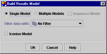
Once a model has been partitioned, a new model can be created that preserves the highlighting colors. A new model can is created by first pressing the Build Results Model… button that will display the build results model dialog shown in figure 8.5a.

Building a single results model with the build results model dialog settings shown in figure 8.5a will create a new VDL model with the colors assigned by the partitioning process and open it in the VDL Browser. The new model will be identical to the model shown in figure 8.4.

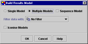
Building a multiple results model with the build results model dialog settings shown in figure 8.5b will create five new VDL models, each containing the units with the colors assigned by the partitioning process. Figure 8.6 shows the five new VDL models that will be created.

Figure 8.4 – The multiple partition of the UK Terrain model.

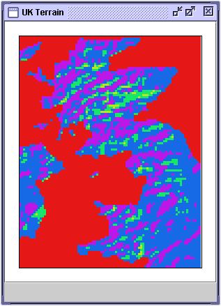
Figure 8.5 – The Build Results Model dialog.

(a)

(b)

(c)

Figure 8.6 – The five models produced after partitioning the UK Terrain model.

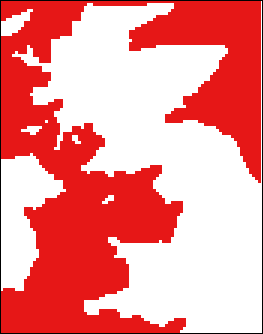
(a) Partition model 1: Sea.

(b) Partition model 2: land 4.

(c) Partition model 3: land 3.

(d) Partition model 4: land 2.

(e) Partition model 5: land 1.

The Sequence Model option enables a multiple results model to be created as a sequence model (figure 8.5c). Each new model will be contained in a group with a sequence layout. Each group contains the units with the colors assigned by the partitioning process. Figure 8.7 shows the controls provided to view and manipulate the sequence model.

Figure 8.7 – The sequence model window of the multiple partitioned UK Terrain model.

8.6 Partitioning the New Hampshire Model

The New Hampshire model that will be used to demonstrate partitioning.

Partitioning Values

The values of the county-name data tag of the New Hampshire model will be used to illustrate the partitioning of values. The Partition tool settings shown in figure 8.8 will enable the model to be partitioned using the county-name XML data tag. Figure 8.9 shows the New Hampshire model partitioned by county name. All of the units have been assigned one of the colors in the partition key. Each color represents one value of the county-name data tag. For example, all of the units with the county-name data tag value Grafton are colored cyan.

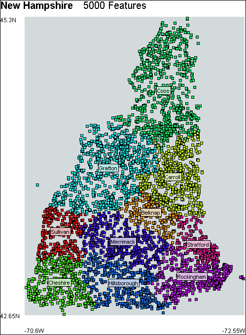
Clicking on the Label button will label each partition as shown in figure 8.10. The text of each label is the name of the partition, either a value or a numeric range.

Figure 8.8 – The Partition tool dialog settings for partitioning the New Hampshire model by county name.

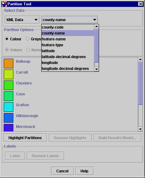
Figure 8.9 – The New Hampshire model partitioned by county name.

Figure 8.10 – The New Hampshire model with labelled county-name partitions.

Partitioning Numeric Ranges

The values of the longitude-decimal-degrees data tag of the New Hampshire model will be used to illustrate partitioning into numeric ranges. The Partition tool settings shown in figure 8.11 will enable the model to be partitioned using the longitude-decimal-degrees XML data tag. Figure 8.12 shows the New Hampshire model partitioned using the longitude of the features. All of the units have been assigned one of the colors in the partition key, based on which partition the value of the longitude-decimal-degrees field falls into. Clicking on the Label button will label each partition as shown in figure 8.13.

Figure 8.11 – The Partition tool dialog settings for partitioning the New Hampshire model into numeric ranges of the longitude of the features.

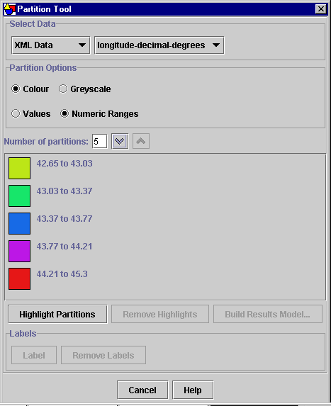
Figure 8.12 – The New Hampshire model partitioned into numeric ranges of the longitude of the features.

Figure 8.13 – The New Hampshire model with labelled numeric-range partitions.

9. The Zoom Tools

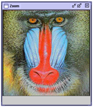
The zoom tools enable models to be explored by zooming in and out. The zoom in tool enables the user to zoom into a unit. Clicking on a unit will cause its visual presentation to be smoothly animated by simultaneously changing is position, scale and orientation. The position is changed from its current position to the centre of the model window. If the unit has been scaled, the scale is changed so that the visual presentation fills the model window. The orientation is also changed so that it is in standard position.

Figure 9.1a shows a unit with an image visual presentation scaled to be half its size and oriented about its centre by 90 degrees anti-clockwise.

<unit>
   <presentation>
      <visual type="image" url="file:c:/images/mandrill.gif" border="true" />
      <scaling scale="0.5" />
      <orientation about="centre" angle="-90" />
   </presentation>
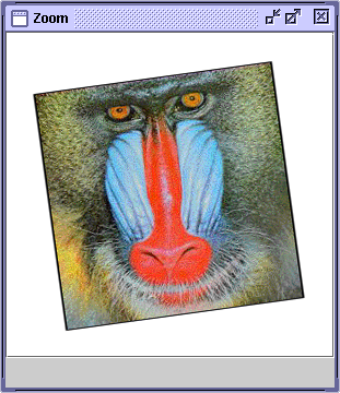
</unit>

Clicking on the image with the zoom in tool will smoothly animate the image by scaling and rotating it so that it fills the window in standard position. Figures 9.1b and 9.1c show two of the intermediate animation stages and figure 9.1d shows the final result. Clicking on the image with the zoom out tool reverses the zoom in animation by smoothly zooming out to display the entire model (figure 9.1a).

Figure 9.1 – Clicking on a unit with the Zoom In tool smoothly animates the unit into standard position to fill the model window.

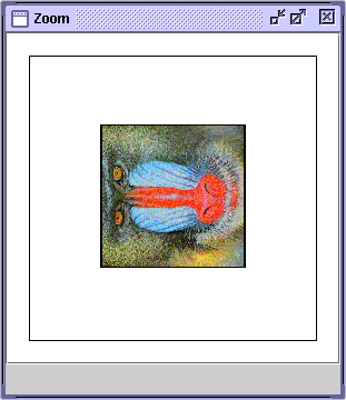
(a)

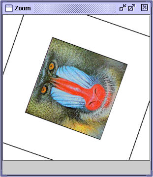
(b)

(c)

(d)

10. The Navigation Tool

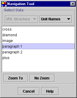
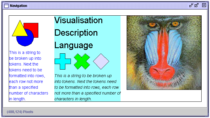
The Navigation tool enables users to zoom to the viewpoints in a model. The Navigation tool is displayed with Tools>Navigation Tool. Figure 10.1 shows the Navigation Tool dialog for the Navigation model shown in figure 10.2a. The Navigation model contains a number of unit and group viewpoints.

<unit viewpoint="paragraph 1">
   <presentation>
      <visual type="text" columns="20" color="blue" fontSize="14"
              fontStyle="plain">
          This is a string to be broken up into tokens. Next the tokens need
          to be formatted into rows, each row not more than a specified number
          of characters in length.
      </visual>
   </presentation>
</unit>

<group viewpoint="shapes">
   <presentation>
      <layout type="row" xSpacing="10" />
   </presentation>
   ...
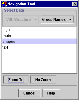
</group>

The Navigation tool has a select data are that is identical to the select data areas of the Browse and Partition tools (see section 7.1). The value selected by the combo box determines whether the names of unit or group viewpoint are displayed. Figure 10.1a shows the viewpoint names of the units and figure 10.1(b) shows the viewpoint names of the groups.

Viewpoints are navigated to by selecting the name of a viewpoint from the list in the Navigation tool dialog and pressing the Zoom To button. The navigation tool uses the same smooth animation as the zoom tools described in section 10. The Zoom Out reverses the zoom in animation by smoothly zooming out to display the entire model (figure 10.2a).

Figure 10.2b shows the Navigation model after zooming in on the viewpoint called shapes as shown in figure 10.1b. Figure 10.2c shows the Navigation model after zooming in on the viewpoint called paragraph 1 as shown in figure 10.1a.

Figure 10.1 – The Navigation tool dialog.

(a) Unit names

(b) Group names

Figure 10.2 – Navigating around the Navigation model.

(a)

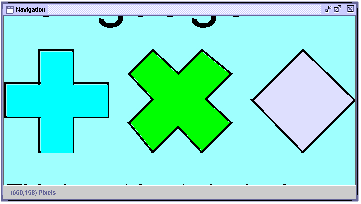
(b)

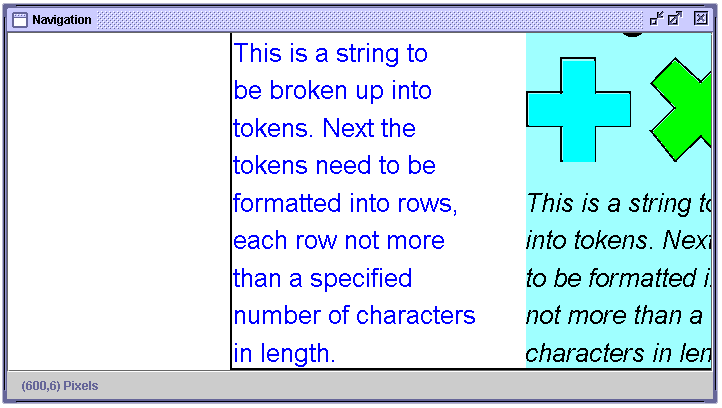
(c)

11. The Sequence Model Editor Tool

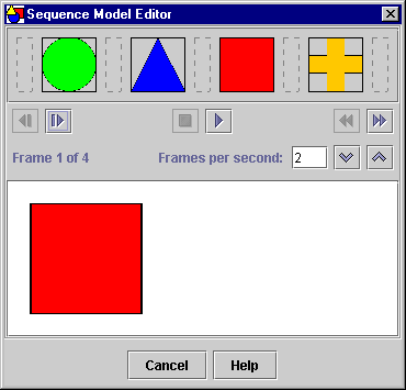
The Sequence Model Editor enables the order of the frames in a sequence model to be re-arranged. The Sequence Model Editor tool is displayed with Edit>Edit Sequence Model and is shown in figure 11.1. The top half of the Sequence Model Editor tool shows each frame in the sequence. The bottom half contains the controls provided by a sequence model window.

Figure 11.1 – The Sequence Model Editor tool.

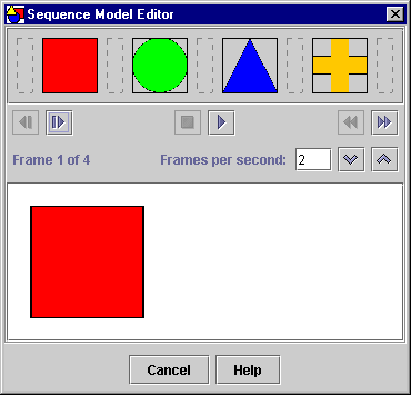
The sequence model shown in figure 11.1 has four frames, each frame is a unit with a colored standard visual presentation. The order of the frames is changed by dragging the frame onto the dashed grey rectangle to the left and right of each frame. The dashed rectangles are the positions where a frame can be inserted. As the frame is dragged over an insertion point, a red I-beam cursor is displayed to provide the user with feedback that shows the frame can be dropped. Figure 11.2(a) shows the red I-beam cursor that is displayed when the frame with the red square is dragged and dropped in between the frames with the blue triangle and orange cross. Figure 11.2(b) shows that the position of the frame with the red square has been changed.

Figure 11.2 – Changing the position of a frame in a sequence.

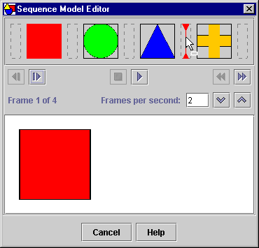
(a)

(b)