
VDL Filters
- Introduction
- Filtering Data
- Example Filters
- The Space Filler Filter
- The Sequence Filter
- The Cache Matrix Chart Filter
- The Cache Bar Chart Filter
- The Document Matrix Chart Filter
- The Document Bar Chart Filter
- The Geographical Names Information Service (GNIS) Filter
1. Introduction
The Visualization Description Language (VDL) is an XML tag-based language for describing interactive visualizations. VDL visualizations or models are implementation language independent visual descriptions of data.
This document describes how data is processed with VDL filters to create VDL models. Several example VDL filters are also described.
2. Filtering Data
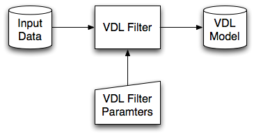
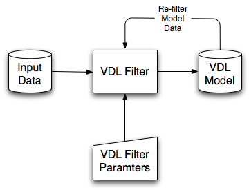
VDL filters take raw input data, process that input and generate a VDL model of the data. Figure 2.1 shows the production of a VDL model with a VDL filter. The input data is passed to the VDL filter. The user specifies the parameter values of the filter and the filter generates the VDL model. The VDL Browser provides the main environment and user interface for VDL filters.
Figure 2.1 – Filtering and re-filtering data to produce a VDL model.
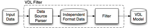
A VDL filter is composed of a Data Source Parser component and a Filtering component. The Data Source Parser component parses the data in the input data file and transforms it into a data source independent format. The Filtering component generates a VDL model from the data source independent format data. Figure 2.2 shows the anatomy of a VDL filter.
Figure 2.2 – The components of a VDL filter.
The data source independent data format is a set of tagged XML data that will be enclosed between the data tags of a unit or group. Table 1.1 shows an example of a data source. Each row of the table describes a person.
Table 1.1 – An example input data source.
| First Name | Last Name | Date of Birth | Height |
|---|---|---|---|
| John | Smith | 28-09-65 | 1.82 |
| Robert | Jones | 19-03-72 | 1.71 |
| Sarah | Peterson | 03-08-69 | 1.34 |
The Data Source Parser component generates the data in an input source marked up in a XML tags. The data in table 1 can be marked up in several ways. The data might be marked up to preserve the data exactly as it appears in the table as shown in figure 2.3a. Some data values such as the name might be joined as shown in figure 2.3b. The data might also be processed, for example to calculate the age of the person as shown in figure 2.3c.
Figure 2.3 – The first row of data shown in table 1 marked up in XML data tags.
<first-name>John</first-name>
<last-name>Smith</last-name>
<birth>29-09-65</birth>
<height>1.82</height>
(a)
<name>John Smith</name>
<birth>29-09-65</birth>
<height>1.82</height>
(b)
<first-name>John</first-name>
<last-name>Smith</last-name>
<age>36</age>
<height>1.82</height>
(c)
The tagged data shown in figure 2.3 would then be attached to a unit or group by enclosing it in the data tags of a unit or group.
<unit>
   ...
   <data>
      <first-name>John</first-name>
      <last-name>Smith</last-name>
      <birth>29-09-65</birth>
      <height>1.82</height>
   </data>
</unit>
Many different visualizations can be made of the same set of data. Many different VDL filters can therefore be created to produce them. Once a Data Source Parser component has been developed it can be re-used to produce different VDL filters for the same input data.
2.1 Inputting Data
The first stage of filtering data is passing the input data to the VDL filter. There are two methods of passing data to a VDL filter:
- through user interaction
- programmatically
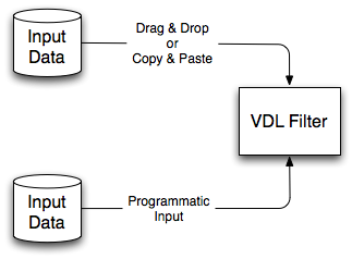
Users input data to a VDL filter by drag and drop or copy and paste operations. Data can also be input to a VDL filter programmatically using the VDL Filter API. Figure 2.4 shows the two methods of inputting data to a VDL filter.
Figure 2.4 – Inputting data to a VDL filter.
2.1.1 User Interaction Input
Software such as the VDL Browser enables users to interact with VDL filters. Users interact with two types of filters:
- copy and paste filters; and
- drag and drop filters
Both types of filter have an icon. Copy and paste filters are presented as push buttons with the icon as the label of the button. Figure 2.5a shows the Scatter Plot filter as an example of a copy and paste filter. The input to a copy and paste filter is the data on the clipboard. Users select appropriate data for the filter in an application and click the filter button. The data shown in table 1 could be stored in an application such as spreadsheet that can be copied and pasted into a filter.
Drag and drop filters are presented as an icon onto which input data files and directories are dragged. Figure 2.5b shows the Space Filler filter as an example of a drag and drop filter. Users drag a file or directory with appropriate content for the filter onto the icon. The data shown in table 1.1 could be stored in a formatted text file that can be dragged onto a filter.
Figure 2.5 – VDL filter icons.

(a) The push button of a copy and paste filter.

(b) The label of a drag and drop filter.
The sequence of interactions with a copy and paste filter is as follows:
- User: Copy the input data onto the clipboard.
- User: Click the push button of the filter.
- Computer: Display a filter parameter dialog if there are any parameters.
- User: Set the parameter values and press the OK button.
- Computer: Validate the filter parameter values and display error messages if appropriate.
- Computer: Generate a VDL model.
The sequence of interactions with a drag and drop filter is as follows:
- User: Drag the input data file or directory onto the filter.
- Computer: Display a filter parameter dialog if there are any parameters.
- User: Set the parameter values and press the OK button.
- Computer: Validate the filter parameter values and display error messages if appropriate.
- Computer: Generate a VDL model.
2.1.2 Programmatic Input
The copy and paste and drag and drop operations are the user interfaces to VDL filters. Data can be inputted programmatically to all VDL filters using the VDL Filter API. Programmatic input enables data to be passed through a filter in code without requiring interaction from the user. The copy and paste and drag and drop operations are built using programmatic input.
2.2 Filter Parameters
Any VDL filter can have parameters that control how the input data is transformed into a VDL model. VDL filter parameters can be one of several data types:
- string;
- integer;
- double;
- Boolean; or
- enumerated values.
Enumerated values are a list of string values from which one must be selected.
Each filter parameter is described by the name of the parameter and its data type. The software that contains the filter is responsible for capturing the values of the parameters from the user. This involves displaying the parameters names and collecting the values of the parameters from the user.
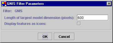
The parameters of filters contained in standard applications such as the VDL Browser will be displayed in a dialog. A parameter dialog is displayed when the user either copies data into a filter or drags a file onto a filter. Figure 2.6 shows the parameters for the Geographical Names Information Service (GNIS) VDL filter. The GNIS filter has an integer parameter that controls the size of the model and a Boolean parameter that controls whether geographical features should be displayed as icons or as data points. This dialog therefore captures an integer value and a Boolean value.
When parameters are presented in an application dialog, string, integer and double parameter values are entered into an input box. Boolean parameter values are presented as a check box. Enumerated values are presented as options selected with a combo box.
Figure 2.6 – The GNIS filter parameter dialog.
2.3 Re-Filtering Data
The ability to re-filter data is an important characteristic of VDL filters. All or a selection of the data in a model can be passed through a VDL filter to create a new model. Different parameter values can be set to produce a different view of a set of data. Re-filtering a selection of data enables that selection to be examined more closely. Re-filtering data is a key feature of the VDL Browser.
VDL filters have two characteristics that enable them to re-filter data:
- VDL filters can accept data selected from any VDL model that it produced.
- VDL filters can accept data selected from any VDL model produced by a different filter, if that filter processes the same data.
New VDL models can be produced by passing all or part of the data in an existing VDL model through a filter. Figure 2.7 shows the production of a new model by re-filtering the data in an existing model. The user selects the data to re-filter and the selected data is passed through the filter. The user specifies the parameter values of the filter (if any) and the filter generates a new VDL model.
Figure 2.7 – Re-filtering data to produce a VDL model.
Filters process tagged data so re-filtering involves passing tagged data extracted from a model through the filter. The filtering component does not and cannot make any distinction between tagged data produced by parsing an input data source and tagged data selected and extracted from an existing model.
3. Example Filters
VDL filters are developed with the VDL Filter API. Any VDL filters can be plugged into the VDL Browser.
The following are examples of VDL filters and their icons:
 |
Space Filler Filter |
 |
Sequence Filter |
 |
Cache Matrix Chart Filter |
 |
Cache Bar Chart Filter |
 |
Document Matrix Chart Filter |
 |
Document Bar Chart Filter |
 |
Geographical Names Information Service (GNIS) Filter |
4. The Space Filler Filter
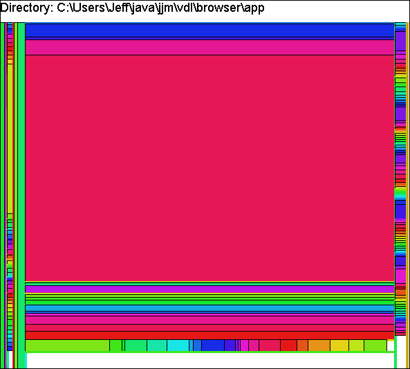
The Space Filler filter takes a directory as input and generates a Space Filler visualization of the files in that directory. A Space Filler visualization shows each file is a directory structure as a colored rectangle. The area of the rectangle is proportional to the size of the file. Space Filler visualizations enable large files to be identified quickly and easily. A description of Sneiderman’s Space Filler Treemap visualization can be found at the University of Maryland’s Human Computer Interaction Lab.
The Space Filler filter has three parameters:
- the width of the model (in pixels)
- the height of the model (in pixels)
- whether the rectangles representing files are in color or greyscale
Figure 4.1 shows the Space Filler filter parameters as presented by the VDL Browser. Figure 4.2 shows a Space Filler visualization.
Figure 4.1 – The Space Filler filter parameter dialog.
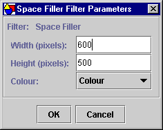
Figure 4.2 – A Space Filler filter visualization.
5. The Sequence Filter
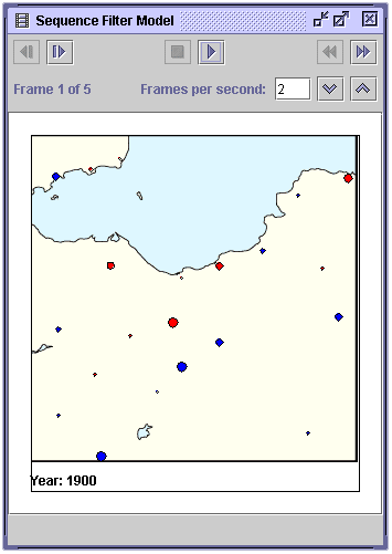
The Sequence filter is a compositing filter that is useful for building movies of data that changes over time. It takes as input a directory containing VDL model files. The Sequence filter sorts the files by the date of last modification and builds a new model. The new model contains a group with a sequence layout. The sequence group will contain one group for each of the models in the directory.
The images in figure 5.1 are VDL models that present the population of several towns and cities around Edinburgh, UK between 1900 and 1940. Towns are represented by blue circles and cities are represented by red circles. The size of the population of the towns and cities is represented by the diameter of the circles; the larger the population, the greater the diameter of the circle.
Figure 5.1 – Five VDL models to be made into a sequence model.
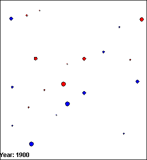
(a) Frame 1.
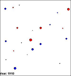
(b) Frame 2.
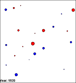
(c) Frame 3.
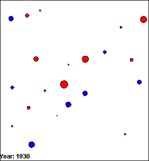
(d) Frame 4.
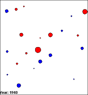
(e) Frame 5.
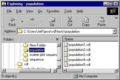
The VDL models shown in figure 5.1 are each stored in the population directory shown in figure 5.2. The construction of each model in figure 5.1 is similar to that of the Edinburgh Region model. Dragging the population directory onto the sequence filter icon produces the sequence model shown in figure 5.3. In this model a background image of the Edinburgh region has been added to complete the model.
Figure 5.2 – The five Edinburgh population VDL model files listed in Microsoft Explorer.
The sequence model shown in figure 5.3 can be exported as QuickTime or AVI format movies by selecting File>Export As>QuickTime Movie and File>Export As>AVI Movie, respectively, in the VDL Browser.
Figure 5.3 – The Edinburgh Sequence model.
6. The Cache Matrix Chart Filter
The Cache Matrix Chart filter produces visualizations of WWW server cache log files as a 2D table of matrix charts. The Cache Matrix Chart filter processes data files containing WWW cache log entries and produces a Matrix Chart visualization of the data.
6.1 Data
Cache log files contain a variety of information about a cached WWW resources. The following is a typical entry in a WWW cache log file:
911219824.040 2707 gateway-brahma TCP_MISS/304 187 GET
   http://www.star.net.cn/starbbs/right.htm bojian DIRECT/www.star.net.cn -
Each entry in the cache log file is parsed to extract the following information:
- URL
- content type
- access method
- resource size
- when the resource was first logged in the cache
- user
The URL is parsed to extract the following information:
- first level domain
- top two domains
- hostless domain
The content type is parsed to extract the following information:
- minor content type
- major content type
This information is then marked up using the following tags:
<url><first-level-domain><top-two-domains><hostless-domain><access-method><resource-size><first-logged><content-type><major-content-type><minor-content-type><user>
The following is an example of a WWW cache log file entry marked up in these tags.
<resource>
   <url>http://channels.real.com/getlatest.glh</url>
   <first-level-domain>com</first-level-domain>
   <top-two-domains>real.com</top-two-domains>
   <hostless-domain>real.com</hostless-domain>
   <access-method>http</access-method>
   <resource-size>8208</resource-size>
   <first-logged>911216704</first-logged>
   <content-type>audio/vnd.rn-realaudio</content-type>
   <major-content-type>audio</major-content-type>
   <minor-content-type>vnd.rn-realaudio</minor-content-type>
   <user>-</user>
</resource>
6.2 Visualization
A matrix chart is a visualization of a 2D table of quantities. Each quantity is represented by a circle; the diameter of the circle is proportional to the size of the quantity.
Figure 6.1a shows a numeric table of quantities that represent the number of journal papers published by two fictitious authors Smith and Jones in the years 1999, 2000 and 2001. Figure 6.1b shows a matrix chart visualization of the same numeric data. In the matrix chart each quantity—the number of papers published—is represented by a filled circle. The diameter of the circles is proportional to the number of papers published. The matrix chart visualization enables the differences between numeric quantities to be seen more easily.
Figure 6.1 – Numeric values presented as a table and as a matrix chart.
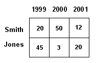
(a) A numeric table.
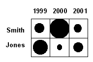
(b) Matrix chart of the numeric table.
The Cache Matrix Chart filter visualizes cache data by producing a 2D table of matrix charts, each element of the table is a matrix chart. The axes of the table each represent a field of the cache data record described above. Every combination of x axis values and y axis values are presented. Each matrix chart represents the data matching an x axis field value and a y axis field value. Some combinations have no matches and are represented by a dash.
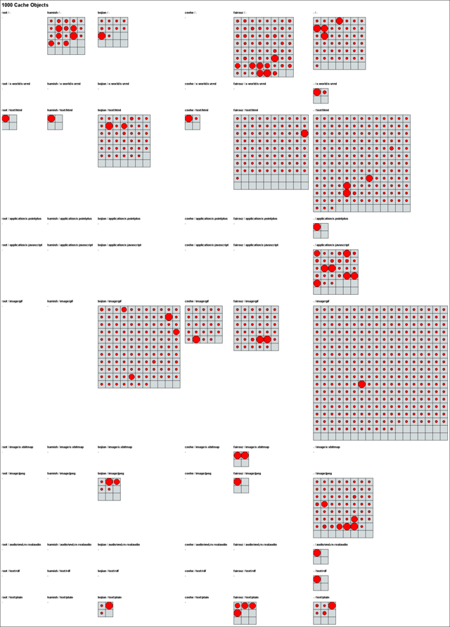
Figure 6.2 shows the Cache Matrix Chart model. In this matrix chart, the x axis represents users and the y axis represents content types. Each matrix chart represents the data for one of the users and one of the content types. The number of cache resources for each combination of x and y axis values can be compared using the size of the matrix charts.
Figure 6.2 – A Cache Matrix Chart model.
The Cache Matrix Chart filter has three parameters:
- The field to represent on the x axis;
- The field to represent on the y axis; and
- The maximum size of each cell (in pixels) which controls the maximum diameter of each circle in the matrix chart.
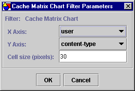
Figure 6.3 shows the Cache Matrix Chart filter parameters as presented by the VDL Browser.
Figure 6.3 – The Cache Matrix Chart filter parameters dialog.
7. The Cache Bar Chart Filter
The Cache Bar Chart filter produces visualizations of WWW server cache log files as a table of bar charts.
7.1 Data
The data processed by the Cache Bar Chart filter is the same as the data processed by the Cache Matrix Chart filter.
7.2 Visualization
The Cache Bar Chart filter visualizes cache data by producing a row of bar charts. Each bar chart shows the frequency of occurrence of the values that occur in one field of the cache data record. One bar chart is shown for each of the following fields of the cache data record:
- first-level-domain;
- top-two-domains;
- hostless-domain;
- content-type;
- major-content-type;
- minor-content-type;
- user; and
- access-method.
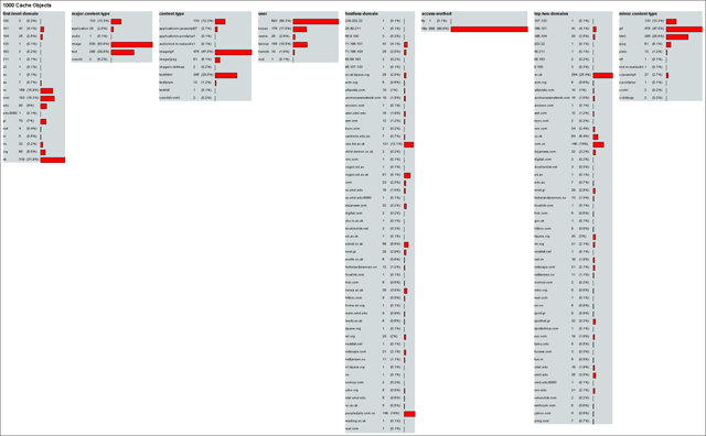
Figure 7.1 shows the Cache Bar Chart model.
Figure 7.1 – A Cache Bar Chart model.
8. The Document Matrix Chart Filter
The Document Matrix Chart filter produces visualizations of document data as a 2D table of matrix charts.
8.1 Data
The Document Matrix Chart filter processes data files containing document records. Each document record contains the following information about each document:
- title
- author(s)
- publication year
- publication type (Journal Article, Book, Conference Paper, etc)
- title of the document in which the document was published (Journal Name, Conference Title, etc, if any)
The input document record file is parsed and this information is marked up using the following tags:
<document>
   <title>Static Dependent Costs for Estimating Program Execution Time</title>
   <author>Reistad, Brian and Gifford, David K.</author>
   <year>1994</year>
   <type>inproceedings</type>
   <booktitle>Conference on Lisp and Functional programming</booktitle>
</document>
8.2 Visualization
The Document Matrix Chart filter visualizes document data by producing a 2D table of matrix charts. The axes of the table each represent a field of the document data record described above. Every combination of x axis values and y axis values are presented. Each matrix chart represents the data matching an x axis field value and a y axis field value. Some combinations have no matches and are represented by a dash.
Figure 8.1 shows a document matrix chart model. In this matrix chart, the x axis represents publication type and the y axis represents publication year. Each matrix chart represents the data for one of the publication types and one of the publication years.
Figure 8.1 – A Document Matrix Chart model.
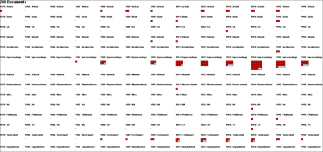
The matrix charts produced by the Document Matrix Chart filter are slightly different to those produced by the Cache Matrix Chart filter. As there is no field in the document data records that contains numeric quantity, each document is represented by fixed size square.
The number of documents for each combination of x and y axis values can be compared using the size of the matrix charts.
The Document Matrix Chart filter has three parameters:
- The field to represent on the x axis
- The field to represent on the y axis
- The maximum size of each cell (in pixels) which controls the width and height of each square in the matrix chart
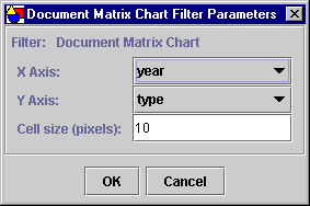
Figure 8.2 shows the Document Matrix Chart filter parameters as presented by the VDL Browser.
Figure 8.2 – The Document Matrix Chart filter parameters dialog.
9. The Document Bar Chart Filter
The Document Bar Chart Filter produces visualizations of document data as a table of bar charts. The Document Bar Chart filter processes data files containing document records and produces a Bar Chart visualization of the data.
9.1 Data
The data processed by the Document Bar Chart filter is the same as the data processed by the Document Matrix Chart filter.
9.2 Visualization
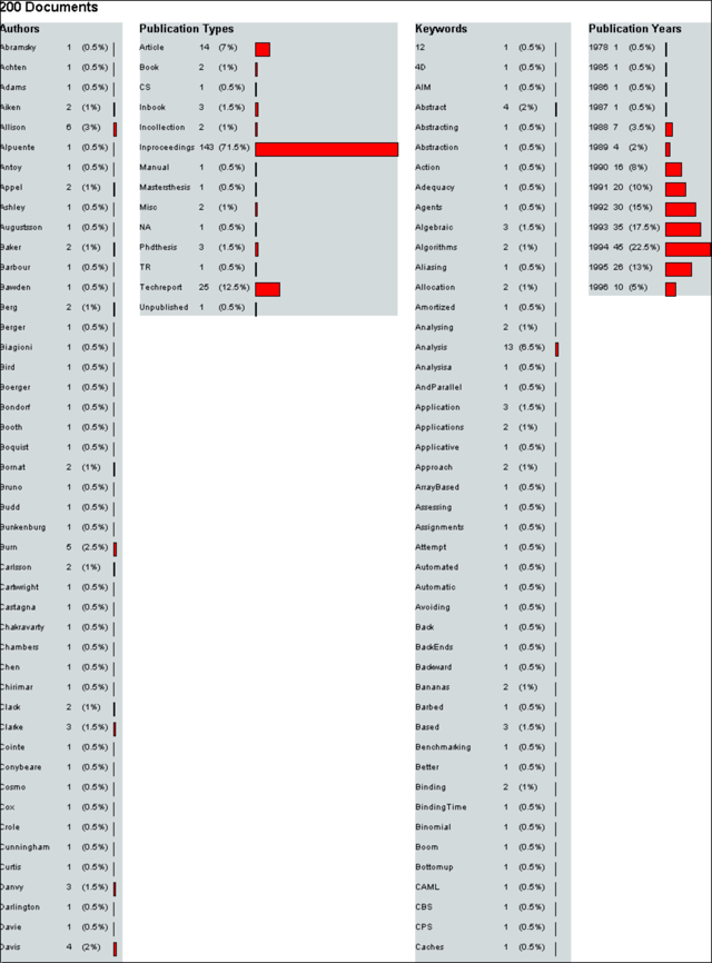
The Document Bar Chart filter visualizes document data by producing a table of bar charts. Each bar chart shows the frequency of occurrence of the values that occur in one field of the document data record. One bar chart is shown for each of the following fields of the document data record:
- author
- publication type
- keywords extracted from the title
- publication year
Figure 9.1 shows a document bar chart model</a>.
Figure 9.1 – A Document Bar Chart model.
10. The Geographical Names Information Service (GNIS) Filter
The Geographical Names Information Service (GNIS) data files describe physical and cultural features of each U.S. state. The GNIS filter processes GNIS data files and produces a scatter plot visualization of those features.
10.1 Data
GNIS data describes named geographical features using a variety of attributes. The GNIS filter uses the following attributes:
- state code;
- feature name;
- feature type;
- county name;
- primary latitude;
- primary longitude;
- primary latitude (decimal degrees); and
- primary longitude (decimal degrees).
The attribute values for each feature are stored in a data file, one file per state. The GNIS data files for each state are available from the U.S. Board on Geographic Names website, which also provides a full description of the GNIS data file format.
The state of New Hampshire will be used to demonstrate the GNIS filter. The extract in table 10.1 shows ten features of the New Hampshire data set. The source data file is parsed and the relevant information is extracted and marked up in the following set of tags.
<GNISDataEntry>
   <state-code>NH</state-code>
   <feature-name>A-Z Trail</feature-name>
   <feature-type>trail</feature-type>
   <county-name>Grafton</county-name>
   <county-code>009</county-code>
   <longitude>441158N</longitude>
   <latitude>0712736W</latitude>
   <longitude-decimal-degrees>44.19944</longitude-decimal-degrees>
   <latitude-decimal-degrees>-71.46</latitude-decimal-degrees>
</GNISDataEntry>
Table 10.1 – An extract from the GNIS data describing New Hampshire.
| State Code | Feature Name | Feature Type | County Name | Latitude | Longitude | Latitude (decimal degrees) | Longitude (decimal degrees) |
|---|---|---|---|---|---|---|---|
| NH | A-Z Trail | trail | Grafton | 441158N | 0712736W | 44.19944 | -71.46 |
| NH | AMC Kingsman Pond Shelter | locale | Grafton | 440815N | 0714359W | 44.1375 | -71.73306 |
| NH | Aaron Ledge | bench | Sullivan | 433211N | 0720108W | 43.53639 | -72.01889 |
| NH | Abbot Hill | summit | Hills-borough | 424756N | 0714430W | 42.79889 | -71.74167 |
| NH | Abbot Hill | summit | Grafton | 441426N | 0713901W | 44.24056 | -71.65028 |
| NH | Abbott Brook | stream | Cheshire | 430555N | 0721201W | 43.09861 | -72.20028 |
| NH | Abbott Brook | stream | Coos | 450853N | 0712133W | 45.14806 | -71.35917 |
| NH | Abbott Brook | stream | Coos | 445617N | 0710151W | 44.93806 | -71.03083 |
| NH | Abbott Memorial Trust Dam | dam | Hills-borough | 425042N | 0714424W | 42.845 | -71.74 |
| NH | Abel Brook | stream | Grafton | 433740N | 0713926W | 43.62778 | -71.65722 |
10.2 Visualization
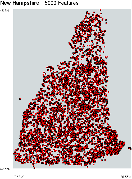
The physical and cultural features are visualized as a scatter plot. The features are presented as red squares at a low level of detail and as icons at a high level of detail. The position of each square is determined by the longitude-decimal-degrees and latitude-decimal-degrees fields. The longitude of a feature is mapped onto the y axis and the latitude is mapped onto the x axis. Figure 10.1 shows the New Hampshire GNIS model.
Figure 10.1 – The New Hampshire model.
The GNIS filter has two parameters:
- the length of the largest dimension of the model (in pixels)
- whether the features are displayed as data points or as icons
The length of largest model dimension (in pixels) parameter controls the size of the scatter plot. The user supplies this length and it determines the length of the x axis if the model is wider than it is tall, or the y axis if the model is taller than it is wide. After the length of the largest dimension is assigned, the length of the other dimension is calculated to maintain the aspect ratio of the data. Figure 10.2 shows the GNIS filter parameters as presented by the VDL Browser.
Figure 10.2 – The GNIS filter parameters dialog.
Features can be displayed at a higher level of detail as icons by checking the Display features as icons parameter. The GNIS filter currently uses GUI application icons1 to represent the physical and cultural features. These are placeholders that will be replaced when a suitable set of geographic icons are found. However, even using the GUI application icons, patterns in the data are highlighted, such as the stream feature which is represented by the information icon in figure 10.3. Figure 10.4 shows four more example models created with the GNIS filter.
Figure 10.3 – Re-filtered New Hampshire model.
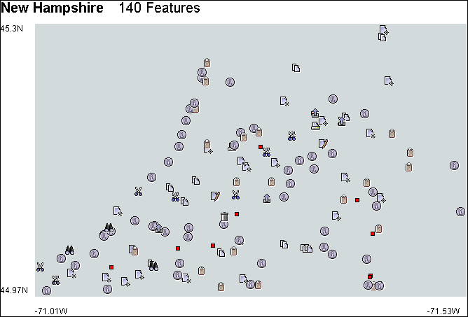
Figure 10.4 – Example GNIS filter models.
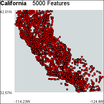
(a) California.
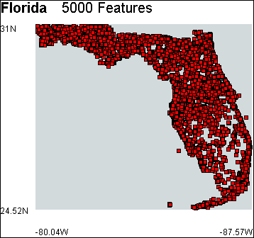
(b) Florida.
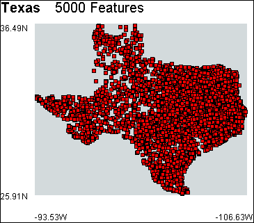
(c) Texas.
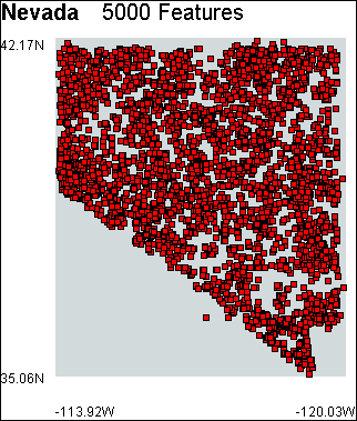
(d) Nevada