A Genetic Algorithm for Feature Labelling in Interactive Applications

This article describes an algorithm for labelling features in interactive applications such as data visualization. In the first phase, a genetic algorithm searches for a set of label positions that minimizes the number of labels that overlap features, other labels, or the bounding box of the region to be labelled. The genetic search has a time limit to ensure that interactive software that uses the algorithm is responsive. If there are any overlapping pixels after the genetic search, the second phase of the algorithm makes small adjustments to the position of the overlapping labels to remove the overlaps.

1. Introduction

This article describes a genetic algorithm for labelling features in bounded regions such as maps. This algorithm is aimed at labelling features in interactive applications such as data visualization.

In the first phase of the algorithm, the genetic algorithm searches for a set of label positions that minimizes the number of labels that overlap features, other labels, or the bounding box of the region to be labelled. The genetic search has a time limit to ensure that interactive software that uses the algorithm is responsive. If there are any overlapping pixels after the genetic search, the second phase of the algorithm makes small adjustments to the position of the overlapping labels to remove the overlaps.

Section 2 describes six established criteria for automated labelling algorithms. Section 3 describes the labels that are positioned by this algorithm, the ways in which these labels can overlap, and the ways that the overlapping is corrected. Section 4 introduces genetic algorithms and section 5 describes the feature labelling genetic algorithm. Section 6 presents a brief evaluation of the labelling algorithm and section 7 concludes with a set of improvements to the current algorithm.

2. Requirements for Automated Labelling Algorithms

Imhof (1962) developed six general requirements for positioning labels that are often cited in the literature on feature labelling algorithms:

1. Readability—the size, font, colour, and position of the labels should support the reader;
2. Definite attachment—it must be clear to which feature a label refers;
3. Avoidance of overlaps—labels should not overlap features or other labels;
4. Spatial integration—the shape of the label should make the type of the label clear;
5. Site identification—the font should indicate the type of feature that is labelled;
6. Overall aesthetics—labels should be positioned to avoid clusters and symmetry.

The algorithm described in this article is aimed at labelling features in interactive applications such as data visualization. Object labelling in interactive applications is often temporary; there is therefore less emphasis on aesthetics than for the permanent labels required for printed maps, for example. The most important requirements for this algorithm are therefore definite attachment and avoidance of overlaps.

The next section describes the labels that are positioned by this algorithm.

3. The Labels

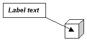
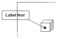
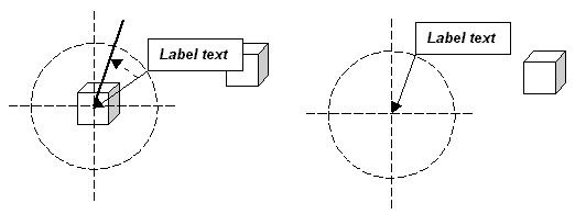
The feature labelling algorithm positions the labels of individual features rather than groups of features. The type of label positioned by this algorithm is shown in below. A rectangular box containing the text of the label points at the centre of the feature with a line with an arrowhead. The definite attachment requirement is met by connecting the label to the feature with this line. The goal of the feature labelling algorithm is to meet the avoidance of overlaps requirement.

3.1 Positioning Labels

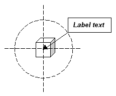
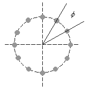
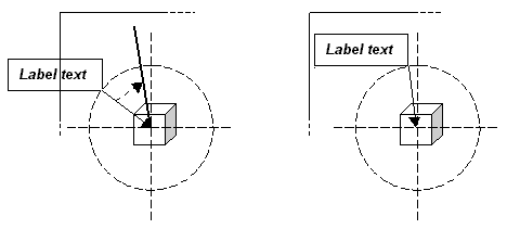
The current position of a label is described by the angle θ of rotation about the centre of a circle centered on the feature (below left). The radius of the circle is the length of the line that connects the corner of the bounding box of the label to the centre of the feature. Labels are positioned by moving the bounding box along the circumference in steps of φ degrees (below right).

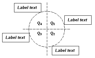
One of the four corners of the bounding box always touches the circumference. The corner that touches the circumference depends on the quadrant of the circle that the bounding box lies in, as shown below. If the bounding box is anywhere along the circumference in quadrant one, the lower left corner of the bounding box touches the circumference; if the bounding box is in quadrant two, the upper left corner touches the circumference, and so on. If the bounding box changes quadrant as it is moved along the circumference, the corner that touches the circumference changes.

3.2 Overlapping Labels

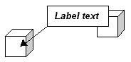
A labelling algorithm needs to position each label so that as few labels as possible overlap. There are three ways in which labels can overlap: labels can overlap the outside of the region bounding box (below left), features (below centre), and other labels (below right). Labels that overlap the bounding box of the region to be labelled are undesirable because the part of the label that is outside the bounding box will be clipped and not seen. Labels that overlap features or other labels are undesirable because they will obscure them.

3.3 Correcting Overlapping Labels

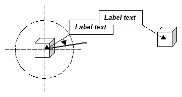
The three overlapping label problems described above are solved by jittering. Jittering moves the bounding box along the circumference until the label no longer overlaps the bounding box, a feature, or another label. The following diagram illustrates the solution to the overlapping bounding box problem: the label is moved clockwise along the circumference until the label is completely inside the region bounding box.

The following illustration demonstrates the solution to the overlapping feature problem: the label is moved anti-clockwise along the circumference until it no longer overlaps the feature.

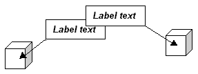
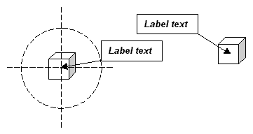
The diagram below shows the solution to the overlapping label problem: the label on the left is moved clockwise along the circumference until it no longer overlaps the label; the label on the right is not moved. Another solution would be to move the label on the right and hold the label on the left still. A third solution would be to move both labels in opposite directions until they no longer overlap. This is more complex but requires the least amount of movement.

Overlapping labels can be corrected by jittering one or at most two labels until they no longer overlap. As the number of labels increases, the complexity of jittering rises exponentially. Jittering alone is an impractical method of positioning labels. For any non-trivial labelling task, there are simply too many labels to move. A solution to the overlapping labels problem that can deal with this complexity is required.

3.4 Restating the Problem

The overlapping labels problem can be restated as an overlapping pixels problem. The pixels of a label can overlap the pixels of features, other labels, and the (imaginary) region outside the bounding box of the region. An algorithm that solves the overlapping pixels problem must minimize the number of overlapping pixels. An ideal solution will be one in which none of the pixels overlap.

Genetic algorithms are particularly well suited for solving the overlapping pixels problem because they are function minimization optimizers that rapidly search the solution space in parallel.

4. Genetic Algorithms

Genetic algorithms (GAs) are a class of learning, search, and optimization algorithms based on the mechanisms of natural selection and natural genetics (Goldberg 1989).

GAs model a problem as a population of individuals; each individual is a single solution to the problem. The goal of a GA is to increase the utility of each successive generation until it has been maximized. The utility of each generation is increased with a survival of the fittest selection mechanism. Each individual is assigned a fitness value that represents how good a solution it is. Individuals are selected according to their fitness value; the higher the fitness value, the greater the probability of an individual contributing one or more offspring to the next generation.

Individuals are composed of their genetic material. New individuals are created by manipulating the genetic material of existing individuals with two genetic operators, crossover and mutation. Crossover exchanges a portion of the genetic material of two parent individuals at a random point to produce two new child individuals. Mutation changes a randomly chosen piece of genetic material.

A typical GA works as follows (based on the description by Forsythe and Rada (1986):

1. generate an initial population of individuals at random;
2. evaluate the fitness of the individuals; if the overall average fitness is good enough stop and display the individuals with the highest fitness;
3. for each individual, compute its selection probability p = f / F where f is the fitness of the individual and F is the total fitness of all the individuals;
4. generate the next population by selecting individuals according to the selection probabilities and applying the genetic operators;
5. repeat from step 2.

The next section describes the feature labelling GA.

5. The Labelling Algorithm

The feature labelling algorithm has two phases: GA search followed by label jittering. In the first phase, the GA searches the solution space to find a set of label positions that minimizes the number of overlapping pixels. If there are any overlapping pixels, the second phase of the algorithm jitters the labels to correct the overlapping, as described in section 3.3.

5.1 Inputs

The GA feature labelling algorithm has four inputs:

1. the dimensions of the bounding box of the region that contains the features;
2. the length of the radius of the circle that is centered on the features;
3. the locations of the features to label;
4. the text and font of the labels.

5.2 The Fitness Function

The GA searches the solution space of label positions with a fitness function that minimizes the number of overlapping pixels. The fitness of each individual is inversely proportional to the number of overlapping pixels in the solution. The lower the number of overlapping pixels, the greater the fitness. The number of overlapping pixels is the sum of all the pixels that overlap features, other labels, and the region outside the bounding box of the region.

5.3 Representation

The position of each label is represented by the angle θ of rotation about the centre of the circle, and is encoded as a binary string of six bits. The value of θ, that ranges from 0 to 359 degrees, is mapped onto a value in the range 0 to 63. This enables θ to be represented in six bits: 2⁶ = 64. Representing θ in six bits reduces the length of each chromosome – 0 to 359 would take nine bits to represent.

The binary strings represent values in the range 0 to 63 and new values created by the crossover operator are also in this range. Mapping from 0 to 63 back to 0 to 359 produces values with an interval of 5.625 (360 / 64 = 5.625) which implements the value φ, the amount by which θ is incremented when the bounding box of a label is moved along the circumference of the circle: φ = 5.625 ≈ 6°.

Six degrees is a useful increment. If the value of θ is too small, the increments in θ will not move the label along the circumference far enough; the next position will be too similar to the previous position and too little progress towards a solution will be made. Similarly, if the increments in θ are too large, the number of positions will be insufficient to enable the labels to be positioned to avoid overlapping.

An individual contains the value of θ for each label. An individual is constructed as follows. For each label:

1. map the angle θ in the range 0 to 359 onto an integer value in the range 0 to 63 to produce θ’;
2. create the string version of θ’ represented in binary as a sequence of characters ‘0’ and ‘1’;
3. append this string to the end of the individual;
4. repeat from step 1 until all label angles have been added.

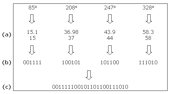
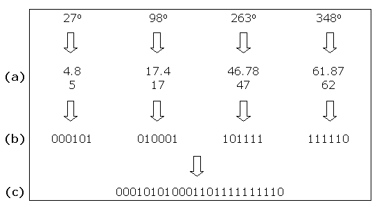
The following diagrams illustrate the creation of two individuals that represent the positions of two sets of four labels: the angle of rotation θ in the range 0 to 359 is mapped onto the range 0 to 63 and rounded up (a); the angle in the range 0 to 63 is converted into a string of six bits (b); all four strings of six bits are concatenated into a 24 bit string (c).

5.4 Genetic Operators

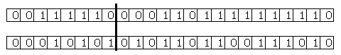
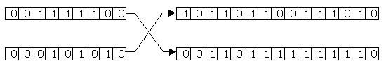
The following diagrams show the creation of two child individuals from two parent individuals. A single-point crossover operator swaps parts of the generic material of two parent individuals to create two child individuals that are added to the next generation. A random crossover point along the length of the string of ‘1’s and ‘0’s is chosen (a); the genetic material to the right of the crossover point is swapped (b) to create two new child individuals (c).

Crossover is applied to every pair of parent individuals because a suitable solution has not yet been found; if one had been found, the algorithm would have terminated.

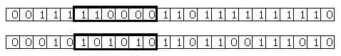
A mutation operator is applied with probability 0.1. A random bit in the string of ‘1’s and ‘0’s is chosen and flipped: a ‘0’ is replaced with a ‘1’ and a ‘1’ is replaced with a ‘0’.

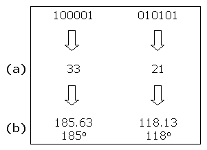
The following diagram shows how these new values are decoded: the six-bit binary strings are converted into an integer in the range 0 to 63 (a); and the integer in the range 0 to 63 is then mapped onto the range 0 to 359 and rounded up (c).

5.5 Running the GA

The GA is run each time a new set of label positions is required. The first step is to create an initial population made up of individuals that represent a set of random label positions. The GA creates new generations of label positions until either the allowed time elapses, or the number of overlapping pixels is minimized, ideally to zero.

The GA has two stopping conditions. The first and most obvious is to stop when there are no more overlapping pixels. In practice, this is generalized to allow a maximum number of overlapping pixels. A small number of overlapping pixels (<30-50) distributed over a set of labels is not noticeable and enables the search to terminate more quickly.

The second stopping condition uses a timer to terminate the search when a specified amount of time has elapsed. The solution returned by the GA is the best that can be found in the time available. A fixed time limit ensures that the labelling algorithm will take the same amount of time on slower machines as on faster machines. The solutions produced by faster machines will be better than those of slower machines because faster machines will be able to search more of the solution space in the time available, but the response times will be the same. Users often prefer an acceptable solution now rather than the best solution later.

Responsiveness is important because labelling is often invoked by a user command, such as a pull-down menu option in an interactive system. Responsiveness is vital when the labelling command is issued in the context of a series of selection and data labelling operations as part of a data exploration session.

A consistent and predictable response time is required to make an interactive system feel responsive. Shneiderman (1998) recommends that common tasks should take no more than two to four seconds. If this labelling algorithm is used in the context of a series of selection and data labelling operations, then the maximum time allowed for the GA search should be less than four seconds.

6. Evaluation

The following screenshots illustrate the label positions for a set of features produced by this algorithm. The features are towns and cities in a visualization application. In this example, the features are tightly packed and provide a good test of the algorithm’s ability to avoid overlaps.

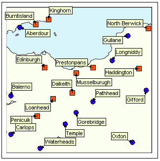
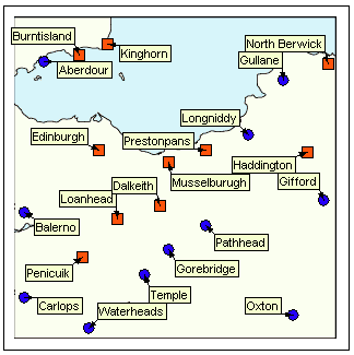
Since the initial placement of the labels—the angle of rotation around the centre of the circle—is random, a different set of label positions will be produced each time the algorithm is run on the same set of features.

7. Improvements

In the current algorithm, the radius of the circle—the length of the line connecting the label to the feature—is fixed. An improvement would be to allow the length of the radius to vary between a minimum and maximum length. This would enable a far greater number of label positions which should make labelling faster. This would be implemented by including the length of the radius as well as the angle of rotation of the label around the circle in the chromosome of each label.

In the current algorithm, all overlapping pixels have the same weight. An improvement would be to weight pixels that overlap features, for example, more heavily than pixels that overlap the region outside the bounding box of the region.

References

• Forsythe, R. and R. Rada, Machine Learning: Applications in Expert Systems and Machine Learning, Ellis Horwood, 1986.
• Goldberg, D. E., Genetic Algorithms in Search, Optimization and Machine Learning, Addison-Wesley, 1989.
• Imhof, E., “Die Anordnung der Namen in der Karte.” In International Yearbook of Cartography, 1962: 93-129.
• Shneiderman, B., Designing the User Interface, Third Edition, Addison-Wesley, 1998.