VDL Models

1. Introduction
2. The UK Terrain Model
3. The Edinburgh Region Model
4. The Computer Network Model
5. The Matrix Chart Model
6. The Bar Chart Model
7. The New Hampshire Model
8. The UK Network Model
9. The Edinburgh Map Model
10. The Aerial Utility Model
11. The Aerial Contour Sequence Model
12. The Orbits Model

1. Introduction

The Visualization Description Language (VDL) is an XML tag-based language for describing interactive visualizations. VDL visualizations or models are implementation language independent visual descriptions of data.

This document describes example visualizations that have been created with VDL. The purpose of each visualization and how it was constructed with VDL is described.

2. The UK Terrain Model

The UK Terrain model shows how a detailed model of a geographical area can be created in VDL. Each individual square tile on the model contains information about the area represented by that tile and can be examined. Figure 2.1 shows the UK Terrain model.

Figure 2.1 – The UK Terrain model.

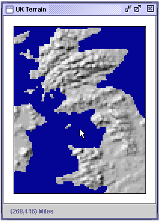
2.1 Presentation

Each square tile is either colored blue to represent the sea, or a shade of grey that represents the elevation of the area it represents. The darker the grey, the lower the elevation. The lighter the grey, the higher the elevation. This VDL model has miles as the units and a scale of 0.5 miles per pixel.

<model name="UK Terrain" units="Miles" scale="0.5">
   ...
</model>

Each blue or grey square is a VDL unit with a square visual presentation. As a VDL unit, each square is individually selectable and can have a set of XML data attached to it with the data tag.

There are 9657 units laid out in 111 rows of 87 columns. The units are arranged in a grid layout.

<group name="UK Terrain">
   <presentation>
      <layout type="grid" rows="111" columns="87" />
   </presentation>
   <unit name="tile">
      <presentation>
         <visual type="rectangle" width="3" height="3"
                 color="0:0:150" border="false" />
      </presentation>
      <data>
         <category>sea</category>
         <elevation>490</elevation>
      </data>
   </unit>
   ...
</group>

2.2 Data

Each unit in the UK Terrain model has two data tags that describe the elevation in feet (elevation) and the category of the area it represents (category). The units are divided into five categories, based on their elevation:

• Sea
• Land 1
• Land 2
• Land 3
• Land 4

An example unit is:

<unit name="tile">
   <presentation>
      <visual type="rectangle" width="3" height="3"
              color="180:180:180" border="false" />
   </presentation>
   <data>
      <category>land3</category>
      <elevation>1790</elevation>
   </data>
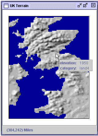
</unit>

Figure 2.2 shows the XML data window for the UK Terrain model displayed in the VDL Browser.

Figure 2.2 – The UK Terrain model data.

3. The Edinburgh Region Model

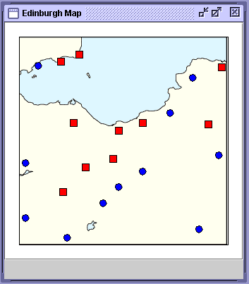
The Edinburgh Region model shows how data points representing towns and cities can be overlaid on an existing image of a map in VDL. This model presents several towns and cities in the area surrounding Edinburgh, UK. Each town and city has information that can be examined. Figure 3.1 shows the Edinburgh Region model.

Figure 3.1 – The Edinburgh Region model.

3.1 Presentation

This model is composed of a unit with an image visual presentation that provides the background map (figure 3.2a), and a set of units with square and circle visual presentations that provide data points representing cities (red squares) and towns (blue circles) in the region (figure 3.2b). The units representing the towns and cities are contained in a group with a position layout and are laid out by specifying the x and y co-ordinates of each unit.

Figure 3.2 – Breakdown of the Edinburgh Region model.

<unit name="Edinburgh Map">
   <presentation>
      <visual type="image"
              url="file:c:/images/Edinburgh.gif"
              border="false" />
   </presentation>
</unit>

(a) VDL describing the background map unit.

<group name="Cities">
   <presentation>
      <layout type="position" />
   </presentation>
   <unit name="Kinghorn">
      <presentation>
         <position x="80" y="20" />
         <visual type="rectangle"
                 width="10" height="10"
                 color="red" border="false" />
      </presentation>
      ...
   </unit>
   ...
</group>

(b) Sample of VDL describing the town and city data points.

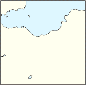
(c) The background image.

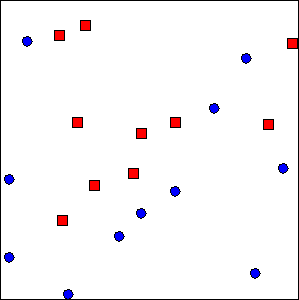
(d) The units representing the towns and cities.

The unit providing the background image and the group containing the units representing the towns and cities are contained in a group with an overlay layout. The group representing the towns and cities are overlaid on top of the unit providing the background image. The towns and cities are overlaid on top of the background because the background occurs before the towns and cities in the group with an overlay layout.

<group name="Edinburgh">
   <presentation>
      <layout type="overlay" />
   </presentation>
   <unit name="Edinburgh Map">
      <presentation>
         <visual type="image" url="file:c:/Edinburgh.gif" border="false" />
      </presentation>
   </unit>
   <group name="Cities">
      <presentation>
         <layout type="position" />
      </presentation>
      <unit name="Kinghorn">
         <presentation>
            <position x="80" y="20" />
            <visual type="rectangle" width="10" height="10"
                    color="255:0:0" border="yes" />
         </presentation>
         <data>
            <place>
               <name>Kinghorn</name>
               <population>100</population>
            </place>
         </data>
      </unit>
      ...
   </group>
</group>

3.2 Data

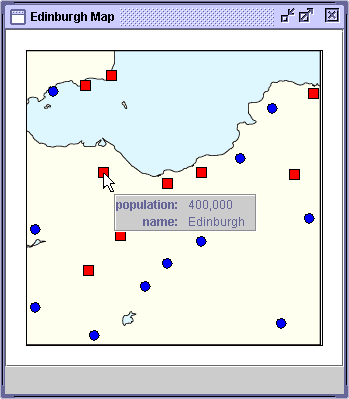
Each unit representing a town or city has XML data that describes it. In this model, each town and city is described by two tags that record its name and population with the name and population tags, respectively.

<data>
   <place>
      <name>Kinghorn</name>
      <population>100</population>
   </place>
</data>

Figure 3.3 shows the XML data window for the Edinburgh Region model displayed in the VDL Browser.

Figure 3.3 – The Edinburgh Region model data.

4. Computer Network Model

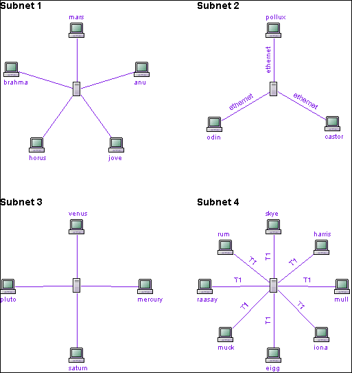
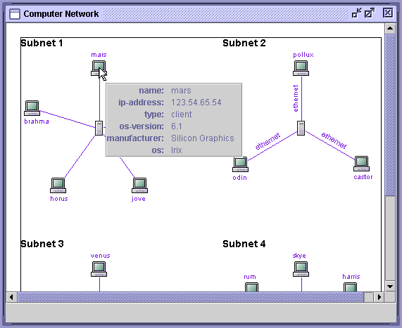
The Computer Network model shows how a set of units can be linked together to model a network of computers. The computers and the links between them have data that can be examined. Figure 4.1 shows the Computer Network Model.

Figure 4.1 – The Computer Network model.

4.1 Presentation

The Computer Network model shows four small example subnets of a university department. Each subnet contains a set of client machines linked to a server.

Each subnet is represented by a group and the four groups are arranged in a 2 x 2 grid layout with 50 pixel spacing between the rows and columns.

<group>
   <presentation>
      <layout type="grid" rows="2" columns="2" xSpacing="50" ySpacing="50" />
   </presentation>
   <group name="Subnet 1">
      ...
   </group>
   <group name="Subnet 2">
      ...
   </group>
   <group name="Subnet 3">
      ...
   </group>
   <group name="Subnet 4">
      ...
   </group>
</group>

Each subnet group contains a unit for the title and a group containing the units that represent the clients, servers and the links between them.

The title of the subnet is a unit with a string visual presentation.

<unit>
  <presentation>
    <visual type="string" value="Subnet 1" color="black"
            fontSize="14" fontStyle="bold" />
  </presentation>
  ...
</unit>

Each client machine is a unit with an image visual presentation.

<unit name="mars">
   <presentation>
      <visual type="image" url="file:c:/vdl/Host24.gif" border="false" />
   </presentation>
   ...
</unit>

The name of the machine is produced by a unit with a string visual presentation.

<unit>
   <presentation>
      <visual type="string" value="mars" color="125:22:229"
              fontSize="10" fontStyle="plain" />
   </presentation>
</unit>

The string and image units are composed in a column layout.

<group>
   <presentation>
      <layout type="column" ySpacing="0" />
   </presentation>
   <unit>
      <presentation>
         <visual type="string" value="mars" color="125:22:229"
                 fontSize="10" fontStyle="plain" />
      </presentation>
   </unit>
   <unit name="mars">
      <presentation>
         <visual type="image" url="file:c:/vdl/Host24.gif" border="false" />
      </presentation>
      ...
   </unit>
</group>

The groups containing the units representing the client machines and their names are arranged in a group with an arc layout.

<group>
   <presentation>
      <layout type="arc" width="200" height="200" extentAngle="360" />
   </presentation>
   ...
</group>

The server machine in each subnet is connected to the client machines with a unit with a link visual presentation. In the following extract, the link connects the unit with the name loki to the unit with the name mars. The link has the label ethernet and both the link and its label are colored magenta.

<group>
   <presentation>
      <layout type="position" />
   </presentation>
   <unit name="link">
      <presentation>
         <visual type="link" from="loki" to="odin"
                 label="ethernet" color="125:22:229" />
      </presentation>
      ...
   </unit>
   ...
</group>

4.2 Data

Three elements of the Computer Network model have data that can be examined:

1. the subnet title;
2. the computers; and
3. the connections between computers.

4.2.1 Subnet Title Data

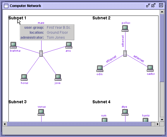
The title of each subnet has data that describes the subnet. Three tags provide the subnet’s location in the building (location), the name of it’s system administrator (administrator), and the group of users assigned to the computers (user-group).

<unit>
   <presentation>
      <visual type="string" value="Subnet 1" color="black"
              fontSize="14" fontStyle="bold" />
   </presentation>
   <data>
      <subnet>
         <location>Ground Floor</location>
         <administrator>Tom Jones</administrator>
         <user-group>First Year B.Sc.</user-group>
      </subnet>
   </data>
</unit>

Figure 4.2 shows the XML data window for the subnet title data of the Computer Network model displayed in the VDL Browser.

Figure 4.2 – The XML data windows for the Computer Network model.

4.2.2 Computer Data

The units representing each computer have six tags that describe the machine’s name (name), whether the computer is a client or a server (type), its IP address (ip-address), its manufacturer (manufacturer), the name (os) and version (os-version) of its operating system.

<unit name="mars">
   <presentation>
      <visual type="image" url="file:c:/vdl/Host24.gif" border="false" />
   </presentation>
   <data>
      <name>mars</name>
      <type>client</type>
      <ip-address>123.54.65.54</ip-address>
      <manufacturer>Silicon Graphics</manufacturer>
      <os-version>6.1</os-version>
      <os>Irix</os>
   </data>
</unit>

Figure 4.3 shows the XML data window for the computer data of the Computer Network model displayed in the VDL Browser.

Figure 4.3 – The XML data windows for the Computer Network model.

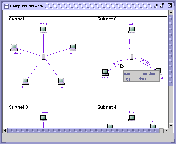
4.2.3 Connection Data

The server machine in each subnet is connected to the client machines with a unit with a link visual presentation. In the following extract, the link connects the unit with the name loki to the unit with the name mars. The link has the label ethernet and both the link and its label are colored magenta.

<unit name="link">
   <presentation>
      <visual type="link" from="loki" to="odin"
              label="ethernet" color="125:22:229" />
   </presentation>
   <data>
      <name>connection</name>
      <type>ethernet</type>
   </data>
</unit>

Figure 4.4 shows the XML data window for the connection data of the Computer Network model displayed in the VDL Browser.

Figure 4.4 – The XML data windows for the Computer Network model.

5. The Matrix Chart Model

The Cache and Document Matrix Chart filters produce matrix chart models.

5.1 Presentation

Figure 5.1 shows a large matrix chart model. The large matrix chart is composed of a number of matrix charts laid out in a grid. The matrix chart model is organised as a group with a column layout. The column contains a unit with a string visual presentation for the title, 1000 Cache Objects, and a group with a grid layout that contains the matrix charts.

<group>
   <presentation>
      <layout type="column" ySpacing="10" />
   </presentation>
   <unit>
      <presentation>
         <visual type="string" value="1000 Cache Objects" color="0:0:0"
                 fontSize="20" fontStyle="bold" />
      </presentation>
   </unit>
   <group>
      <presentation>
         <layout type="grid" rows="11" columns="6" xSpacing="20" ySpacing="20" />
      </presentation>
      ...
   </group>
</group>

Figure 5.1 – The cache matrix chart model.

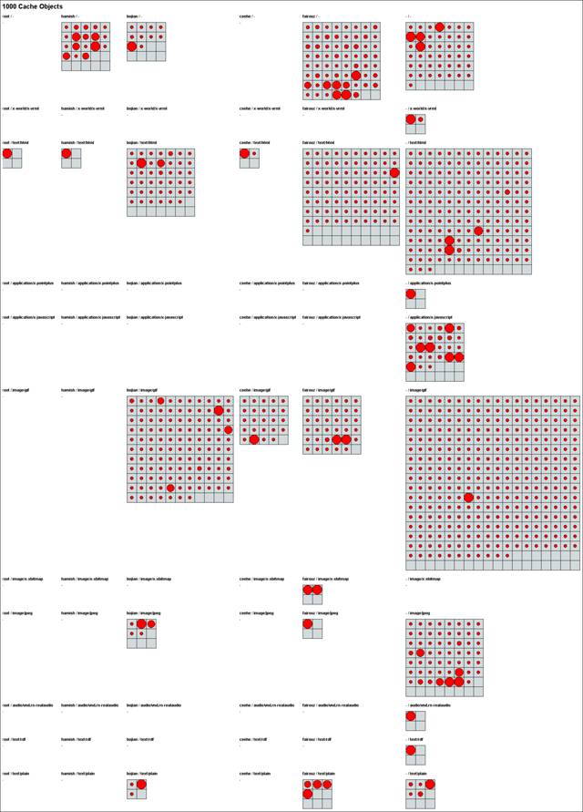
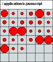
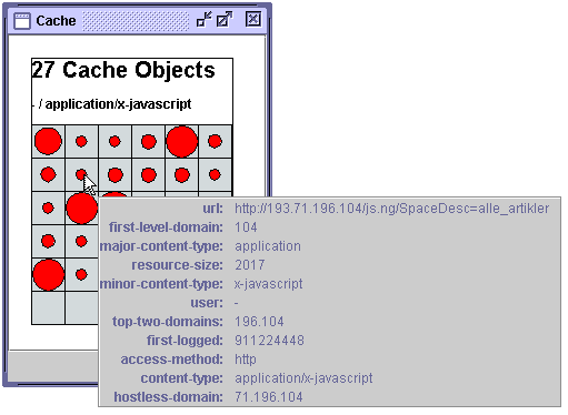
Figure 5.2 shows a single matrix chart in more detail. The matrix chart is contained in a group with a column layout. The group contains the title of the matrix chart, -/application/x-javascript, and the matrix chart is contained in a group with a position layout and a grey background.

<group>
   <presentation>
      <layout type="column" ySpacing="10" />
   </presentation>
   <unit>
      <presentation>
         <visual type="string" value="-/application/x-javascript" color="0:0:0"
                 fontSize="12" fontStyle="bold" />
      </presentation>
   </unit>
   <group background="211:218:220">
      <presentation>
         <layout type="position" />
      </presentation>
      ...
   </group>
</group>

The matrix chart is composed of units with ellipse visual presentations to create the circles. Each circle is laid out by specifying the x and y co-ordinates of the origin of the ellipse visual presentation.

<group background="211:218:220">
   <presentation>
      <layout type="position" />
   </presentation>
   <unit>
      <presentation>
         <position x="10" y="10" />
         <visual type="ellipse" width="10" height="10" color="red"
                 border="true" />
      </presentation>
      ...
   </unit>
   ...
</group>

The lines that form the grid of each matrix chart are created by a path visual presentation with a set of line tags.

<unit>
   <visual type="path" penSize="1" color="black">
      <path>
         <line x1="30" y1="0" x2="30" y2="60" />
         ...
      </path>
   </visual>
</unit>

Figure 5.2 – A single matrix chart from the Cache Matrix Charts Model.

5.2 Data

Each unit has a data tag that describes the data represented by the circle. The following example shows the data for models produced by the Cache Matrix Chart filter.

<unit>
   <presentation>
      <position x="10" y="10" />
      <visual type="ellipse" width="10" height="10" color="red" border="true" />
   </presentation>
   <data>
      <url>http://www.sun.com/template/sunstyle.css</url>
      <first-level-domain>com</first-level-domain>
      <major-content-type>-</major-content-type>
      <resource-size>1639</resource-size>
      <user>hamish</user>
      <minor-content-type>-</minor-content-type>
      <top-two-domains>sun.com</top-two-domains>
      <first-logged>911216704</first-logged>
      <access-method>http</access-method>
      <content-type>-</content-type>
      <hostless-domain>sun.com</hostless-domain>
   </data>
</unit>

Figure 5.3 shows the XML data window for the Cache Matrix Chart model shown in figure 5.2 displayed in the VDL Browser.

Figure 5.3 – The Cache Matrix Chart model data.

6. The Bar Chart Model

The Cache and Document Bar Chart filters produce bar chart models.

6.1 Presentation

Figure 6.1 shows a large bar chart model. The large bar chart is composed of a number of bar charts laid out in a row. The bar chart model is organised as a group with a column layout. The column contains a unit with a string visual presentation for the title, 1000 Cache Objects, and a group with a row layout that contains the bar charts.

<group>
   <presentation>
      <layout type="column" ySpacing="10" />
   </presentation>
   <unit>
      <presentation>
         <visual type="string" value="1000 Cache Objects" color="0:0:0"
                 fontSize="20" fontStyle="bold" />
      </presentation>
   </unit>
   <group>
      <presentation>
         <layout type="row" xSpacing="25" />
      </presentation>
      ...
   </group>
</group>

Figure 6.1 – The Cache Bar Chart model.

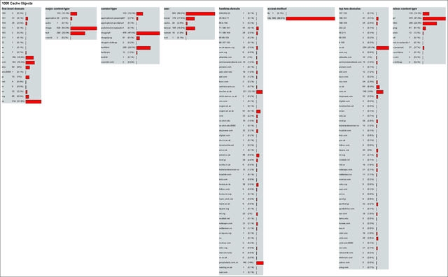
Figure 6.2 shows a single bar chart in more detail. The bar chart is contained in a group with a grey background. The group contains the title of the bar chart, major-content-type, and the bar chart arranged in a column layout.

<group>
   <presentation background="211:218:220">
      <layout type="column" ySpacing="10" />
   </presentation>
   <unit>
      <presentation>
         <visual type="string" value="major-content-type" color="0:0:0"
                 fontSize="16" fontStyle="bold" />
      </presentation>
   </unit>
   <group>
      ...
   </group>
</group>

Figure 6.2 – A single bar chart from the Cache Bar Charts model.

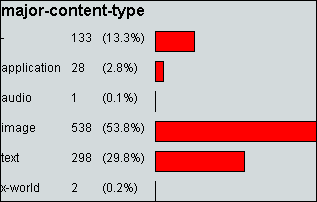
The bar chart itself is implemented as a group of units arranged in a 6 x 4 grid layout. The textual parts are provided by string visual presentations. The bars are provided by rectangle visual presentations that are colored red and have a border.

<group>
   <presentation>
      <layout type="column" ySpacing="10" />
   </presentation>
   <unit>
      <presentation>
         <visual type="string" value="1000 Cache Objects" color="0:0:0"
                 fontSize="20" fontStyle="bold" />
      </presentation>
      </unit>
      <group>
         <presentation>
            <layout type="row" xSpacing="25" />
         </presentation>
         <group>
            <presentation background="211:218:220">
               <layout type="column" ySpacing="10" />
            </presentation>
            <unit>
               <presentation>
               <visual type="string" value="major-content-type" color="0:0:0"
                       fontSize="16" fontStyle="bold" />
            </presentation>
         </unit>
         <group>
            <presentation>
               <layout type="grid" rows="6" columns="4" xSpacing="10"
                       ySpacing="10" />
            </presentation>
            <unit>
               <presentation>
                  <visual type="string" value="-" color="0:0:0"
                          fontSize="12" fontStyle="plain" />
               </presentation>
            </unit>
            <unit>
               <presentation>
                  <visual type="string" value="133" color="0:0:0"
                          fontSize="12" fontStyle="plain" />
               </presentation>
            </unit>
            <unit>
            <presentation>
               <visual type="string" value="(13.3%)" color="0:0:0"
                       fontSize="12" fontStyle="plain" />
            </presentation>
         </unit>
         <unit>
            <presentation>
               <visual string="rectangle" width="39" height="20"
                       color="255:0:0" border="true" />
            </presentation>
         </unit>
      </group>
   </group>
</group>

6.2 Data

The models produced by the Cache Bar Chart filter and the Document Bar Chart filter do not contain any XML data.

7. The New Hampshire Model

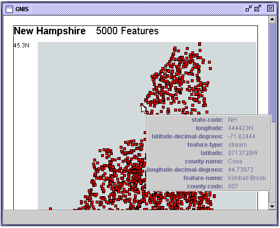
The New Hampshire model was created by the Geographical Names Information Service (GNIS) filter. The New Hampshire model shown in figure 7.1 presents 5000 physical and cultural features of New Hampshire, USA.

Figure 7.1 – The New Hampshire model.

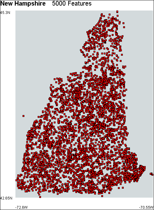
7.1 Presentation

Each physical and cultural feature is presented as a data point presented as a red square. The data points are contained in a group with a position layout and a grey background. The data points are positioned by assigning the x and y co-ordinates. Each data point is presented by a unit with a rectangle visual presentation.

<group>
   <presentation Background="211:218:220">
      <layout type="position" />
   </presentation>
   <unit>
      <presentation>
         <position x="247" y="248" />
         <visual type="rectangle" width="5" height="5" color="red"
                 border="true" />
      </presentation>
      ...
   </unit>
   <unit>
      <presentation>
         <position x="185" y="262" />
         <visual type="rectangle" width="5" height="5" color="red"
                 border="true" />
      </presentation>
      ...
   </unit>
   ...
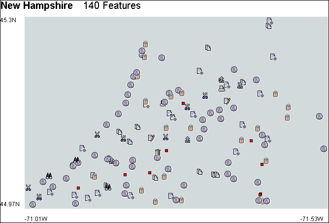
</group>

The GNIS filter can display the physical and cultural features as icons rather than data points to provide a higher level of detail. At this level of detail, each feature is represented by a unit with an image visual presentation. The image is the icon representing the feature. Figure 7.2 shows part of the New Hampshire model with the features displayed as icons.

<unit>
  <presentation>
    <position x="162" y="366" />
    <visual type="image"
            url="file:c:/images/Information16.gif" border="false" />
  </presentation>
</unit>

Figure 7.2 – Part of the New Hampshire model with the feature data points displayed as icons.

The axis labels are provided by units with a string visual presentation. The axis labels are also laid out by assigning the x and y co-ordinates.

<group>
   <presentation>
      <layout type="position" />
   </presentation>
   <unit>
      <presentation>
         <position x="0" y="0" />
         <visual type="string" value="45.3N" color="black" fontSize="12" />
      </presentation>
   </unit>
   <unit>
      <presentation>
         <position x="0" y="600" />
         <visual type="string" value="42.65N" color="black" fontSize="12" />
      </presentation>
   </unit>
   <unit>
      <presentation>
         <position x="50" y="630" />
         <visual type="string" value="-70.6W" color="black" fontSize="12" />
      </presentation>
   </unit>
   <unit>
      <presentation>
         <position x="451" y="630" />
         <visual type="string" value="-72.55W" Colour="black" fontSize="12" />
      </presentation>
   </unit>
   ...
</group>

7.2 Data

Each unit has a data tag that describes the data represented by the square.

<unit>
   <presentation>
      <position x="185" y="262" />
      <visual type="rectangle" width="5" height="5" color="red" Border="true" />
   </presentation>
   <data>
      <state-code>NH</state-code>
      <longitude>440815N</longitude>
      <latitude-decimal-degrees>-71.73306</latitude-decimal-degrees>
      <feature-type>locale</feature-type>
      <latitude>0714359W</latitude>
      <county-name>Grafton</county-name>
      <feature-name>AMC Kingsman Pond Shelter</feature-name>
      <county-code>009</county-code>
      <longitude-decimal-degrees>44.1375</longitude-decimal-degrees>
   </data>
</unit>

Figure 7.3 shows the XML data windows for the New Hampshire model displayed in the VDL Browser.

Figure 7.3 – The XML data windows for the New Hampshire model.

(a)

(b)

8. The UK Network Model

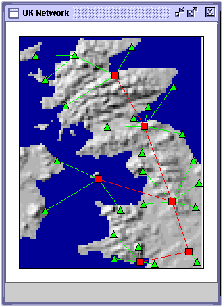
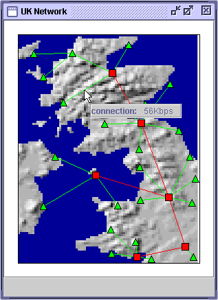
The UK Network model shows how a network structure can be overlaid on another model in VDL. The network represents a set of local stations represented by green triangles linked to hub stations represented by red squares. Local stations are linked by green connections and hub stations are linked by red connections. Figure 8.1 shows the UK Network model.

Figure 8.1 – The UK Network model.

8.1 Presentation

The UK Network model is similar in structure to the Edinburgh Region model. A set of data points connected by links are overlaid on a GIF image of the UK Terrain model. An image of the UK Terrain model was used for simplicity and the actual UK Terrain model could be substituted. The GIF image was produced by choosing File>Export As>GIF Image in the VDL Browser.

The image of the UK Terrain model and the group containing the data points representing the stations are contained in a group with an overlay layout.

<group>
   <presentation>
      <layout type="overlay" />
   </presentation>
   <unit>
      <presentation>
         <visual type="image" url="file:c/images/uk.gif" />
      </presentation>
   </unit>
   <group name="stations">
      <presentation>
         <layout type="position" />
      </presentation>
      ...
   </group>
</group>

Each local stations is represented by a unit with a green triangle visual presentation. Each hub station is represented by a unit with a red rectangle visual presentation. The local and hub stations are contained in a group with a position layout and are laid out by assigning the x and y co-ordinates.

<group name="stations">
   <presentation>
      <layout type="position" />
   </presentation>
   <unit name="Wick">
      <presentation>
         <position x="156" y="10" />
         <visual type="triangle" width="10" height="10"
                 color="green" border="true" />
      </presentation>
      ...
   </unit>
   <unit name="Inverness">
      <presentation>
         <position x="132" y="51" />
         <visual type="rectangle" width="10" height="10"
                 color="red" border="true" />
      </presentation>
      ...
   </unit>
   ...
</group>

The local and hub stations are connected together with units with a link visual presentation. The link visual presentation uses the names of the units it connects to establish the co-ordinates of the end-points of the line representing the connection.

<unit name="Link">
   <presentation>
      <visual type="link" from="Inverness" to="Fort William" Colour="green" />
   </presentation>
   ...
</unit>

8.2 Data

Two elements of the UK Network model have data that can be examined:

• the local and hub stations
• the connections between stations

Local and Hub Station Data

Each local and hub station has two data tags that describe the name of the station (name) and whether it is a local or a hub station (type).

<unit name="Fort William">
   <presentation>
      <position x="61" y="94" />
      <visual type="triangle" width="10" height="10"
              color="green" border="true" />
   </presentation>
   <data>
      <name>Fort William</name>
      <type>local</type>
   </data>
</unit>

Figure 8.2a shows the XML data window for the local station data of the UK Network model displayed in the VDL Browser.

Connection Data

The connections between local and hub stations have a single data tag (connection) describing the speed of the connection between them.

<unit name="Link">
   <presentation>
      <visual type="link" from="Inverness" to="Fort William" Colour="green" />
   </presentation>
   <data>
      <connection>56Kbps</connection>
   </data>
</unit>

Figure 8.2b shows the XML data window for the connection data of the UK Network model displayed in the VDL Browser.

Figure 8.2 – The UK Network model data.

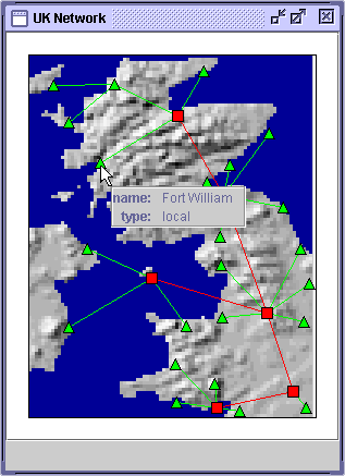
(a) XML data window for a node

(b) XML data window for a connection

9. The Edinburgh Map Model

The Edinburgh Map model shows how a set of icons can be overlaid on an existing map to create an interactive map. Figure 9.1 shows the Edinburgh Map model.

Figure 9.1 – The Edinburgh Map model.

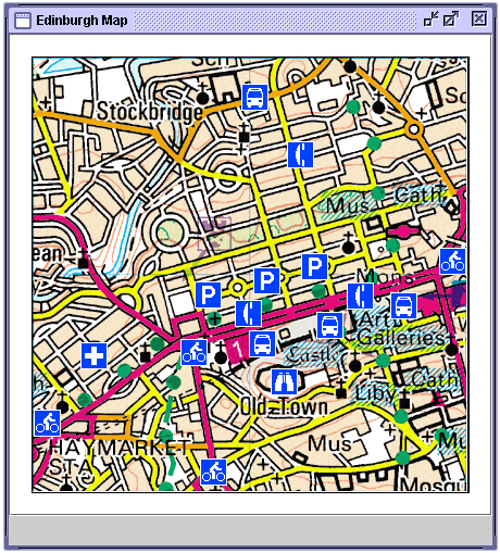
9.1 Presentation

The icons are overlaid on top of a unit with an image visual presentation for the aerial photograph.

<model>
  <group>
    <presentation>
      <layout type="overlay" />
    </presentation>
    <unit name="map">
      <presentation>
        <visual type="image" url="file:c:/images/EdinburghMap.gif"
                border="false" />
      </presentation>
    </unit>
    ...
  </group>
</model>

The icons are produced by an image presentation.

<unit>
   <presentation>
      <visual type="image" url="file:c:/images/phone.gif" border="false" />
   </presentation>
</unit>

9.2 Data

Each icon has data that can be examined to provide the information represented by the icon. The binoculars icon represents a point of interest or an attraction which on this map represents Edinburgh Castle. This icon has three data tags that provide the name of the attraction (attraction), the opening times (opens) and the phone number (phone).

<unit>
   <presentation>
      <position x="220" y="287" />
      <visual type="image" url="file:c:/images/bino.gif" border="false" />
   </presentation>
   <data>
      <attraction>Edinburgh Castle</attraction>
      <opens>Daily, 10:00am - 6:00pm</opens>
      <phone>0131 123 4567</phone>
   </data>
</unit>

The bus icons represent bus stops. Each bus stop icon has a single data tag (routes) that list the numbers of the busses that stop at the bus stop.

<unit>
   <presentation>
      <position x="330" y="217" />
      <visual type="image" url="file:c:/images/busstop.gif" border="false" />
   </presentation>
   <data>
      <routes>14a, 43, 72, 85</routes>
   </data>
</unit>

The parking icons represent car parks. Each car park icon has three data tags that provide parking charge (charge), the times when the charges are applicable (active) and whether the car park is a parking meter or pay and display (type).

<unit>
   <presentation>
      <position x="150" y="207" />
      <visual type="image" url="file:c:/images/park.gif" border="false" />
   </presentation>
   <data>
      <type>Parking Meter</type>
      <charge>1 pound / hour</charge>
      <active>Monday - Saturday, 8:00am - 6:00pm</active>
   </data>
</unit>

Figure 9.2 shows three of the XML data windows for the Edinburgh Map model displayed in the VDL Browser.

Figure 9.2 – The Edinburgh Map model data.

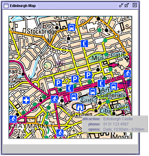
(a) XML data window for a visitor attraction

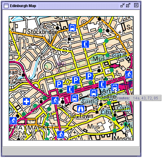
(b) XML data window for a bus stop

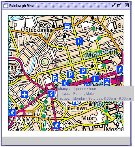
(c) XML data window for a car park

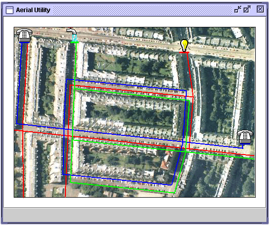
10. The Aerial Utility Model

The Aerial Utility model shows how VDL objects can be overlaid on top of a photograph to add information. The Aerial Utility model shows the location of the wires and pipes of three utilities: telephone, water and electricity. Figure 10.1 shows the Aerial Utility model.

Figure 10.1 – The Aerial Utility model.

10.1 Presentation

The icons and the lines that represent pipes are overlaid on top of a unit with an image visual presentation for the aerial photograph.

<group>
   <presentation>
      <layout type="overlay" />
   </presentation>
   <unit name="map">
      <presentation>
         <visual type="image" url="file:c:/images/Aerial.gif" Border="false" />
      </presentation>
   </unit>
   <group name="Water">
      ...
   </group>
   <group name="Electricity">
      ...
   </group>
   <group name="Telephone">
      ...
   </group>
</group>

The icons are created with an image visual presentation. The lines that representing the pipes and wires are created by a path visual presentation with a set of line tags.

<group name="Telephone">
   <unit>
      <presentation>
         <position x="100" y="0" />
         <visual type="image" url="file:c:/images/Phone.gif" Border="false" />
      </presentation>
      ...
   </unit>
   <unit>
      <visual type="path" penSize="2" color="green">
         <path>
            <line x1="118" y1="118" x2="345" y2="141" />
         </path>
      </visual>
   </unit>
   ...
</group>

10.2 Data

Each of the three icons representing the telephone, water and electricity utilities has data that can be examined. Each utility has four tags that describe whether the utility is telephone, water or electricity (utility), the name of the utility company (company), the region the company is responsible for (region) and the date the pipes or wires were last repaired (last-repaired).

<unit>
   <presentation>
      <position x="5" y="0" />
      <visual type="image" url="file:c:/images/Phone.gif" border="false" />
   </presentation>
   <data>
      <utility>Telephone</utility>
      <company>Central Telecom Ltd.</company>
      <region>Midlands</region>
      <last-repaired>27-5-2001</last-repaired>
   </data>
</unit>

Figure 10.2a shows the XML data window for the utility icon of the Aerial Utility model displayed in the VDL Browser.

Each colored line representing a utility pipe or wire has data that can be examined. Each line has three tags that describe whether the utility is telephone, water or electricity (utility), the depth of the wire or pipe (depth) and the width of the pipe or wire container (width).

<unit>
   <presentation>
      <visual type="path" penSize="1" color="green">
         <path>
            <line x1="118" y1="118" x2="345" y2="141" />
         </path>
      </visual>
   </presentation>
   <data>
      <utility>Water</utility>
      <depth>1.75m</depth>
      <width>0.81m</width>
   </data>
</unit>

Figure 10.2b shows the XML data window for the lines representing utility pipes or wires in the Aerial Utility model displayed in the VDL Browser.

Figure 10.2 – The XML data windows for the Aerial Utility model.

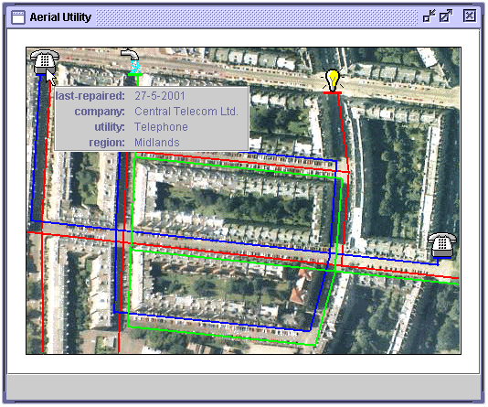
(a) XML data window for a telephone utility

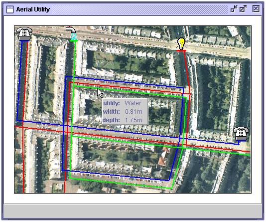
(b) XML data window for a utility pipe

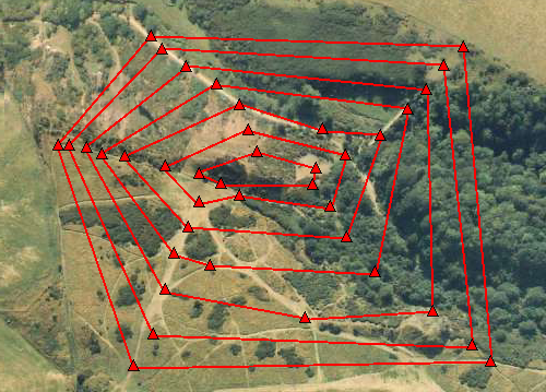
11. The Aerial Contour Sequence Model

The Aerial Contour Sequence model shows how a sequence of VDL objects can be overlaid on top of a photograph to create a movie visualization. Figure 11.1 shows all of the frames of the Aerial Contour Sequence model at the same time. Four of the individual frames are shown in figure 11.3.

Figure 11.1 – The Aerial Contour Sequence model.

11.1 Presentation

The Aerial Contour Sequence model was created by overlaying a group with a sequence layout over a unit with an image visual presentation that provides the aerial photograph.

<model>
   <group>
      <presentation>
         <layout type="overlay" />
      </presentation>
      <unit>
         <presentation>
            <visual type="image" url="c:/images/AerialContour.gif"
                    border="false" />
         </presentation>
      </unit>
      <group name="contours">
         <presentation>
            <layout type="sequence" />
         </presentation>
         ...
      </group>
   </group>
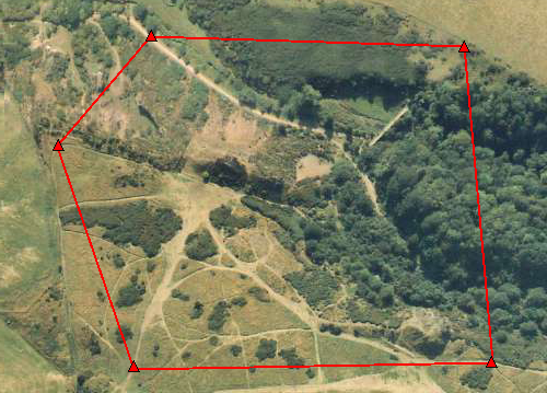
</model>

The group with the sequence layout contains the groups that contain the contour in each frame of the sequence. Figure 11.2 shows four of the contour frames.

<group name="contours">
   <presentation>
      <layout type="sequence" />
   </presentation>
   <group name="frame 1">
      ...
   </group>
   <group name="frame 2">
      ...
   </group>
   ...
</group>

Each contour is made up of a number of triangle and lines. The triangles are created by units with a triangle visual presentation. The lines between the triangles are created by units with path visual presentations.

<group name="frame 1">
   <unit>
      <presentation>
         <visual type="triangle" color="red" border="true" />
      </presentation>
   </unit>
   ...
   <unit>
      <presentation>
         <visual type="path" penSize="1" color="red" />
         <path>
            <line x1="" y1="" x2="" y2="" />
            ...
         </path>
      </presentation>
   </unit>
   ...
</group>

11.2 Data

The Aerial Contour Sequence model has no data.

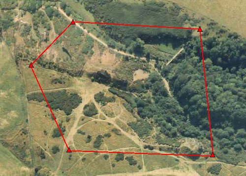
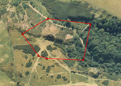
Figure 11.2 – Four of the frames of the Aerial Contour Sequence model.

(a)

(b)

(c)

(d)

Figure 11.3 – Four frames of the Aerial Contour Sequence model overlaid on the aerial photograph.

(a)

(b)

(c)

(d)

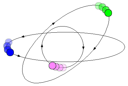
12. The Orbits Model

The Orbits model demonstrates animation with three circles orbiting the same centre point along different elliptical paths (figure 12.1). This model has not been implements because it required VDL behaviors that have not been implemented in the prototype VDL Browser.

Figure 12.1 – The Orbits model.

12.1 Presentation

The orbits model is composed of three orbiting circles. Each one is constructed in the same manner. The circle is constructed from a ellipse visual presentation.

<unit>
   <presentation>
      <visual type="ellipse" width="10" height="10" color="green" border="true" />
   </presentation>
</unit>

The circle unit is contained in a group with an arc layout.

<group name="green">
   <presentation>
      <layout type="arc" width="300" height="200" />
   </presentation>
   <unit>
      ...
   </unit>
</group>

Figure 12.2a show the elliptical path of the arc layout and its rectangular bounding box. The group with the arc layout is rotated counter-clockwise by 30 degrees. An orientation tag is added to the group to rotate the elliptical arc layout.

<group name="green">
   <presentation>
      <layout type="arc" width="300" height="200"
              startAngle="60" extentAngle="360" />
      <orientation about="centre" angle="-30" />
   </presentation>
   <unit>
      ...
   </unit>
</group>

The startAngle attribute of the arc layout specified that the position of the circle will by 60 degrees clockwise from the 12 o’clock position along the elliptical path. Figure 12.2b shows the position of the circle.

Figure 12.2 – The elliptical path.

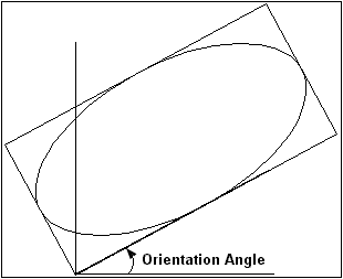
(a) Rotating the elliptical path.

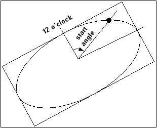
(b) Placing the first unit on the elliptical path.

The animation of the circle around the circular path is implemented with the clock and interpolator tags.

The speed of the orbit depends on how often the clock ticks and the amount by which the startAngle attribute is incremented. The direction of the orbit is controlled by the sign of the amount added to the value of the startAngle attribute.

<group name="green">
   <presentation>
      ...
   </presentation>
   <unit>
      ...
   </unit>
   <clock name="orbitClock" ticks="500" units="milliseconds" />
   <ruleSet>
      <rule>
         <condition event="orbitClock:tick" />
         <action>
            <message>
               <set property="presentation.layout.startAngle"
                    value="presentation.layout.startAngle + 20" />
            </message>
         </action>
      </rule>
   </ruleSet>
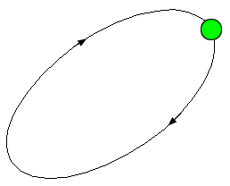
</group>

The clock ticks every half a second which caused the circle to move by 20 degrees along the elliptical path. Figure 12.3 shows the direction of the circle along the elliptical path.

Figure 12.3 – The direction of the animation of the circle along the elliptical path.

Groups for the blue and purple circle orbits are constructed in the same manner as the blue circle orbit. The three groups are composed in an enclosing group with an overlay layout with centre alignment so they will orbit around the same central point.

<group>
   <presentation>
      <layout type="overlay" alignment="centre" />
   </presentation>
   <group name="green">
      ...
   </group>
   <group name="blue">
      ...
   </group>
   <group name="purple">
      ...
   </group>
</group>

12.2 Data

The Orbits model has no data.